Natural and Anthropogenic Influences on the Mount Hope Bay Ecosystem
2006 Northeastern Naturalist 13(Special Issue 4):117–144
The Exchange of Water through Multiple Entrances to the
Mount Hope Bay Estuary
Chris Kincaid*
Abstract - Results are presented from a set of hydrographic surveys conducted within
Mount Hope Bay, RI, during the summer of August, 1996. This sub-system of
Narragansett Bay is interesting because it has two connections to the ocean and it has a
source of thermal energy from the Brayton Point Power Plant. Data was collected on
water velocity, salinity and temperature on days with relatively high ( 2 m range) and
relatively low ( 1 m range) tidal forcing. Velocity data were collected along fixed
transect lines defining the boundaries of the estuary and at fixed stations. Results show
that flow through each of the oceanward entrances has significant horizontal and
vertical structure. The source of fresh water is the Taunton River to the north, and at
times, exchange through this interface exhibits vertically sheared flow. Exchange is
dominated by flow through the interface with Narragansett Bay, where transports reach
3000 m3/s and 6000 m3/s under conditions of low and high amplitude tidal forcing,
respectively. Peak velocities exceed 100 cm/s. Values for transport though the smaller
of the two salt water connections, with the Sakonnet River, and the fresh water entrance,
at the interface with the Taunton River, were 10– 20% of those through the interface
with Narragansett Bay. Velocities are relatively sluggish in the shallow northern shelf
region of the estuary, peaking at < 10 cm/s and 20 cm/s for the low and high tidal
amplitude sampling periods, respectively. Temperature and salinity data reveal significant
levels of stratification and suggest three end-member water sources including a
deep Narragansett Bay source (cold, salty), a shallow river source (warm, fresh) and a
source of water from the Brayton Point region (hot, intermediate salinity). A plug of
warm water that evolves on the northern shelf over the ebb cycle of the tide is advected to
the east–northeast into the shipping channel during the flood. Phase differences in total
instantaneous transport through the two mouths of the system suggest that interactions
with the Sakonnet River are dominated by the greater volume and efficiency of
exchange with the East Passage of Narragansett Bay. Lateral variations in residual
transport show East Passage water entering Mount Hope Bay through the deep central
portion of the cross-section and exiting through confined regions along the edges of the
interface. The pattern in residual exchange with the Sakonnet River shows water exiting
and entering Mount Hope Bay through the western and eastern portions of the cross
section, respectively. A conceptual model is suggested in which these lateral flow
patterns combine with strong vertical mixing in the Sakonnet River Narrows to pump
thermal energy downward in the water column and back northward into the bottom
waters of Mount Hope Bay.
Introduction
Narragansett Bay represents an important ecosystem and resource for the
states of Rhode Island and Massachusetts. Stress levels on the Narragansett
*Graduate School of Oceanography, University of Rhode Island, South Ferry Road,
Narragansett, RI 02882; kincaid@gso.uri.edu.
118 Northeastern Naturalist Vol. 13, Special Issue 4
Bay estuary have been rising. The system is experiencing a period of warming
as evidenced by increasing winter–spring temperature (T) (by as much as
2 °C) that has been attributed to climate trends (Hawk 1998). Recent field
surveys show that the upper portion of the estuary is subject to periods of
chronically low dissolved oxygen (DO) and eutrophication (Deacutis 1999).
Results from intensive summertime sampling through the Narragansett Bay
Estuarine Program at 75 stations within the upper half of Narragansett Bay
suggest that residence times within key regions of the upper Bay, rather than
simply stratification levels, contribute to the evolution of hypoxic events.
The geometry of the estuary is complex. The entrance is composed of
two distinct north–south oriented branches referred to as the East and West
Passages. The upper Bay is comprised of three distinct sub-regions: Greenwich
Bay, the Providence River, and the Mount Hope Bay (MHB) estuary.
Mean depths in this system are relatively shallow, ranging from 7.6 to 10 m
(Pilson 1985a). The deepest portion is the East Passage, with a mean water
depth of 18 m and a maximum water depth of > 40 m. Freshwater enters the
upper Bay through the Providence River, which is fed by the Blackstone and
Pawtuxet Rivers. Another important freshwater source is through MHB,
which is fed by the Taunton River (Fig. 1). The total discharge typically
varies between a minimum of 20 m3/s in late summer–fall to greater than 300
m3/s under peak runoff conditions during the winter–spring months (Pilson
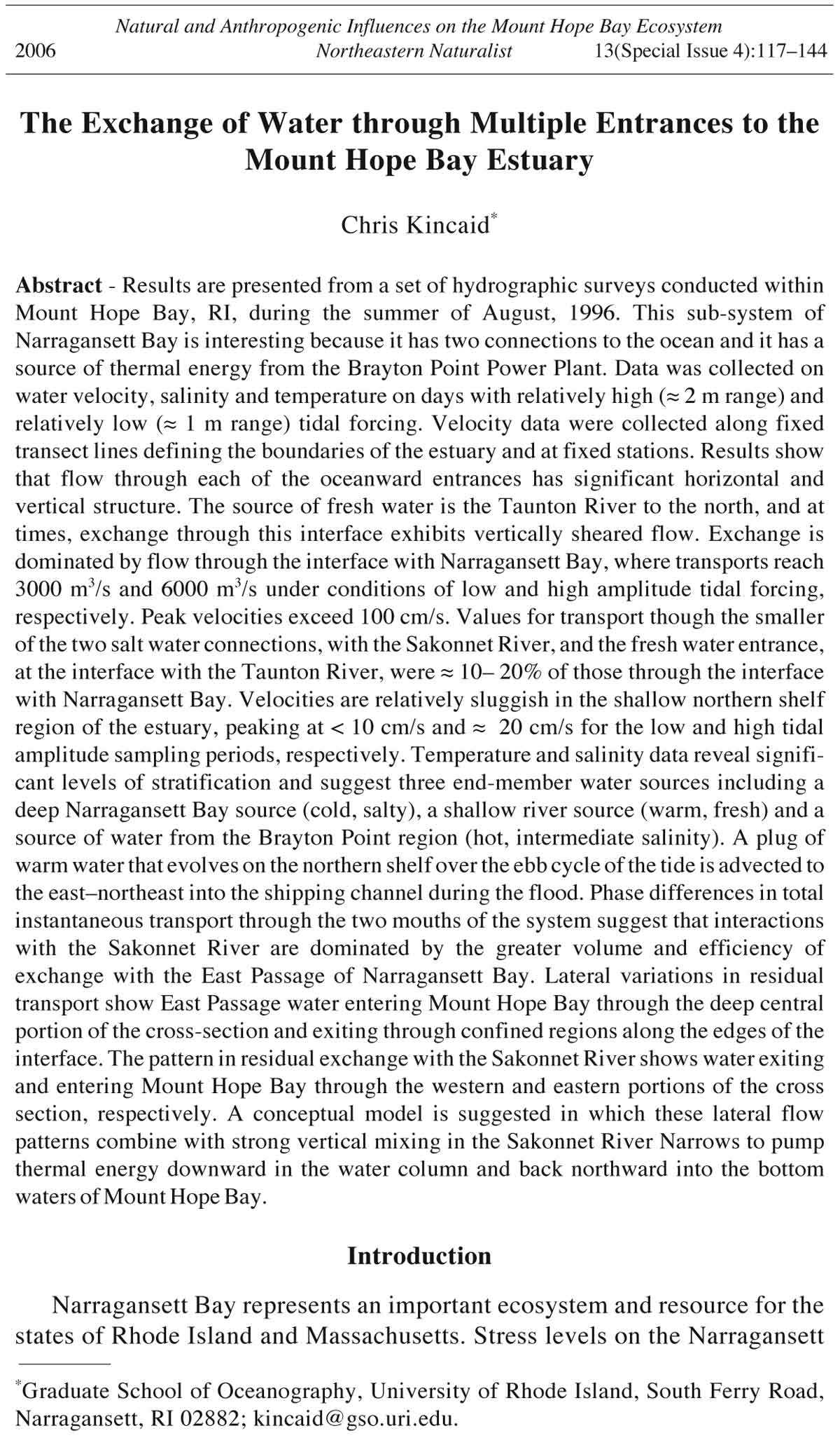
Figure 1. Map of
the Mount Hope
Bay (MHB) estuary
showing the
locations of the
ADCP transect
lines that cross the
entrances to MHB
(T1, T2, and T4).
Another transect
line crosses near
Brayton Point
(T3). Symbols S1,
S2, and S3 mark
locations where
time series data
were collected.
The inset shows
the location of
MHB relative to
Narragansett Bay.
2006 C. Kincaid 119
1985a). The MHB system is of particular interest because it has two connection
pathways to the ocean, one through the East Passage and the other
through the Sakonnet River via the highly constricted and turbulent
Sakonnet River Narrows (SRN) (Levine and Kenyon 1975; Fig. 1).
Over the past 40 years, numerous studies have focused on the physical,
biological and chemical processes within the Narragansett Bay system
(Hicks 1959; Keller et al. 1999; Pilson 1985a,b). Narragansett Bay is characterized
as a partially to well-mixed estuary (Goodrich 1988) that is subject to
strong tidal and wind forcing (Weisburg and Sturges 1976). Maximum
vertical salinity (S) gradients have been estimated to be 2–3 psu (Goodrich
1988, Hicks 1959). Previous modeling and observational studies have focused
on the tidal and wind driven flow (Deleo 2001, Gordon and Spaulding
1987, Hicks 1959, Levine and Kenyon 1975, Spaulding and White 1990,
Weisberg 1976, Weisberg and Sturges 1976). Circulation in the upper Bay
has been shown to be driven in roughly equal parts by tidal and wind forcing
(Weisburg 1976). Previous studies also show that wind effects can permeate
the entire water column, highlighting the importance of the wind in net
estuarine circulation and transport patterns in Narragansett Bay (Weisberg
1972, 1976; Weisberg and Sturges 1976).
Results of the recent intensive summertime DO sampling in upper
Narragansett Bay underscore the importance of constraining circulation
patterns within and exchange between distinct sub-regions of the estuary
through a combination of observational and modeling work. Gordan and
Spaulding (1987) used a vertically integrated model to show that wind
and tidal forcing combine to produce a range of flow patterns between
subsections of the Bay. Physical measurements within Narragansett Bay
have primarily utilized moored current meters at a limited number of
locations (Rosenberger 2001, Shonting 1969, Spaulding and White 1990,
Weisberg and Sturges 1976). In our study, we focus on the sub-region of
MHB, which presents an interesting contrast to other regions of the upper
Bay, i.e., Greenwich Bay and the Providence River. Data from current
meter moorings within MHB show that the system is dominated by the
M2 tide at 80–90% of the energy, with a small contribution at the M4
frequency that gives rise to a double-peaked flood and a single-peaked
ebb (Spaulding and White 1990). Tidal amplitudes (e.g., half the total
tidal range) vary from 40 cm at neap conditions to 80 cm for spring
tides. The system exhibits characteristics of a standing wave, with currents
out of phase with variations in surface elevation by 3 hours. Maximum
tidal currents of 20 cm/s, 22 cm/s, and 4.5 cm/s have been reported
by Spaulding and White (1990) for locations near our lines T1, T4, and
T2, respectively (Table 1). More recent time series data on water level
variations across the SRN reveal aspects of the temporal variability in
exchange between the MHB and Sakonnet River systems (Deleo 2001).
We present data from hydrographic surveys conducted within MHB during
summer, or stratified seasonal conditions. We utilized underway acoustic
120 Northeastern Naturalist Vol. 13, Special Issue 4
Doppler current profiler (ADCP) measurements to characterize both spatial
patterns in circulation within MHB and temporal patterns in exchange through
MHB’s two oceanward connections, with the East Passage of Narragansett
Bay and the Sakonnet River (Fig. 1). A number of recent underway ADCP
surveys have provided detailed spatial images of circulation through the
mouths of major estuaries (Valle-Levinson and Lwiza 1995; Valle-Levinson
et al. 1996, 1998; Wong and Münchow 1995), including Narragansett Bay
(Kincaid et al. 2003). Our results show that flow through each of the salt water
interfaces (T1 and T2 in Fig. 1) exhibits significant lateral structure. Layered
flow is recorded through the freshwater interface at line T4, which is
consistent with the findings of Spaulding and White (1990). However, peak
velocities of > 100 cm/s and 50–60 cm/s are significantly higher than previously
reported for the interface with the East Passage (T1) and at the head of
the system (T4), respectively. Volume flux, or transport data through each
interface, shows the dominant exchange pathway to be through the connection
with the East Passage. Transport through the SRN is 10% of that through line
T1 and is seen to reverse direction late in the flood and ebb stages of the tide,
possibly in response to more efficient filling/flushing that occurs though the
T1 boundary (Deleo 2001). Profiles of S and T show that water properties
within MHB may be explained by mixing between three distinct end-member
sources. The combined data set provides important constraints for threedimensional
hydrodynamic models of flow, transport, and residence time
within Narragansett Bay (Bergondo et al. 2003).
Methods
This study utilized a ship-mounted ADCP in combination with conductivity,
temperature, and depth (CTD) profiles. Circulation patterns and energies
were recorded with an RD Instruments Broadband (1200 kHz) ADCP that was
mounted to the side of a 20' skiff. ADCP data were collected along four
distinct transect lines shown in Figure 1. Two of these lines define boundaries
with water bodies that connect through to the ocean, including one along the
interface with the East Passage of Narragansett Bay, beneath the Mount Hope
Bridge (T1) and another along the interface between MHB and the Sakonnet
River (T2) (Fig. 1, Table 1). Water depths exceed 25 m along the centerline of
T1 and are closer to 16 m at the deepest (eastern) portion of T2. A third
Table 1. Summary of ADCP transect and time series station locations.
Latitude Longitude Latitude Longitude Transect Sampling
Name (start) (start) (end) (end) length (m) Area (m2) time (min)
T1 41°38' 39" -71°15'29" 41°38'12" -71°15'13" 850 9550 10
T2 41°39'02" -71°13'11" 41°38'58" -71°12'31" 850 6200 10
T3 41°41'48" -71°10'48" 41°42'28" -71°11'24" 1450 16000 20
T4 41°43'21" -71°09'16" 41°43'28" -71°09'27" 290 2700 5
S1 41°41'54" -71°10'56" 5
S2 41°42'26" -71°11'56" 5
S3 41°42'25" -71°13'10" 5
2006 C. Kincaid 121
transect (T4) defines the approximate boundary between MHB and the
Taunton River (T4). A relatively narrow region of deeper water runs northeasterly
from line T1, eventually necking down into the shipping channel that
continues along this trend towards line T4 and the Taunton River. To the north
and northwest of the shipping channel lies a broad, shallow region, referred to
here to as the northern shelf. A final line (T3) extends across the northern shelf
from the vicinity of the Brayton Point Power Plant at its northwestern end to
the shipping channel at the southeastern end of the transect. Data ensembles
were collected along transect lines with a ping interval of 7 seconds. The
average boat speed was 1 m/s; hence, velocity ensembles were collected every
7 m along track.
Measurements were also collected at fixed stations, where the vessel
position was held constant and ADCP data were recorded continuously over
a 5-minute time interval. These time series measurements were made at
locations (Table 1) designated S1, S2, and S3 in Figure 1. Station S1 is in the
center of the shipping channel at the southeastern end of T3, near buoy
GC11. The other sites, labeled S2 and S3, were located on the northern shelf
to the south and southwest of the Brayton Point Plant. Hydrographic profiles
were made using a Seabird Seacat 19 CTD at each of the time series sites and
at the mid-points of the transect lines. In the case of transect T3, the CTD
casts were taken within the shipping channel.
Measurements were made on each cruise over a 13-hour period to capture
both ebb and flood stages of the semi-diurnal tidal oscillation. Two
cruises were selected to cover periods of relatively low- and high-amplitude
tides. Figure 2 shows the tidal variation within upper Narragansett Bay from
Providence, RI, for the two sampling days (August 22 and 29, 1996). During
the cruises, ADCP and CTD data were collected along each transect line in
sequence, followed by sampling at the time series locations. A complete set
of measurements, or a circuit, generally required 2.25 hours.
A number of processing steps were performed to improve ADCP data
quality and to highlight both instantaneous and residual circulation
Figure 2. Variation in tidal
height at Providence, RI, for
the two survey days (a) August
22, 1996, and (b) August
29, 1996. Numbers on the
plot show the relative timing
of ADCP files for line T1
(listed in Tables 2 and 3).
122 Northeastern Naturalist Vol. 13, Special Issue 4
patterns in the study area. The raw ADCP data included bad ensembles that
appeared as obvious vertical stripes in contour plots of velocity magnitude
and direction, most often associated with acceleration of the instrument
due to wave activity. In particular, the afternoon sea breeze from the
southwest induced significant wave energy in MHB. A low-pass median
filter was used to remove these bad bins, as described in Kincaid et al.
(2003). A range of filter window widths was investigated, from 4–11 data
values. A comparison of values for integrated or total transport (Q in m3/s)
through each transect shows the different filters agree to within 10%.
However, values for Q calculated from filtered data are consistently lower
(by 5–15%) than those determined using the unfiltered data. Results on
instantaneous and residual flows are presented from filtered data that has
been processed with a median filter window of 5 data values, or ensembles,
which corresponds to 30 m in width.
A number of methods have been used to estimate residual or non-tidal
transport (qR) from shipboard ADCP data (Candela et al. 1990, 1992; Foreman
and Freeland 1991; Geyer and Signell 1990; Munchow et al. 1992;
Simpson et al. 1990). In our analysis, residual transport is calculated within
distinct lateral and vertical sub-sections within each transect in order to
characterize spatial patterns in net exchange between MHB and neighboring
bodies of water. The filtered velocity data were rotated into a transectnormal
component, where positive values correspond to northward flow into
the MHB or, in the case of line T4, northeastward flow into the Taunton
River (Fig. 1). Times for individual transects are related to a dimensionless
tidal stage by comparing the start time (ts) of each transect relative to the
predicted times for low tide at Providence, RI. Normalized transect start
time, t*, was calculated using t* = (ts - t1) / (t2 - t1), where t1 and t2 are the
times of predicted low water before and after a particular survey, respectively
(Tables 2 and 3).
The sampled portion of each transect was divided into subregions covering
the upper and lower halves of the cross section and these were then
sub-sectioned into 10 lateral bins of equal width. Values for instantaneous
transport integrated for each bin were calculated as a function of t* using the
expressions
Qs k t u dx dz
i k j
B i
i j i
i k
( , *)
( )
( )/
,
( )
=
+
=
1 1
1
2 1
(1)
and
Q k t u dx dz
i k j B i
B i
i j i
i k
B( , *) (2)
( ) ( )/
( )
,
( )
=
+
=
1 1
2
where ui,j is the filtered, transect-normal velocity for each ADCP data point
(i = columns or ensembles; j = ADCP depth cell number) and dz and dxi are
the height (50 cm) and width ( 7 m) of each ADCP cell. The lateral
boundaries of each subsection (k) are given in the first summation. The
2006 C. Kincaid 123
number of vertical ADCP cells (B[i]) is a function of position along track.
Within the shallower set of bins (Qs), velocity information is integrated from
the surface ADCP cell down to one bin above the mid-depth level. The series
of bottom subsections (Qb) accumulates information from mid-depth down
to the bottom ADCP cell. A residual transport was next determined for each
Table 2. Summary of ADCP and CTD data from survey day 1: August 22, 1996.
Flow Flow Tidal stage
File Time Transport direction magnitude (0.1 = low,
(MHB) Transect (end) (m3/s) (deg.)* (cm/s) 0.5 = high)
1013 T1 6:50 -1375 -0.05372
1014 T2 7:20 330 -0.01343
1015 T3 8:04 170 C: 270 (55); S: 50 C: 12 (12); S: 5 0.045662 Low water
1016 T4 8:15 245 0.060435
1017 S1 8:27 300 (80) 5 (26) 0.076551
1018 S2 8:39 125 9 0.092667
1019 S3 8:50 60 6 0.10744
1020 T1 9:13 1590 0.13833
1021 T2 10:21 -190 0.22965
1022 T3 10:41 725 C: 90 (90); S: 340 C: 5 (17); s:7 0.25651
1023 T4 10:55 150 0.27532 Mid-flood
1024 S1 11:06 10 (60) 2 (20) 0.29009
1025 S2 11:18 60 (135) 8 (2) 0.3062
1026 S3 11:25 10 (60) 6 (6) 0.31561
1028 T1 11:48 1890 0.34649
1029 T2 12:08 250 0.37335
1030 T3 12:38 1050 C:70; S:50 C:20; S:7 0.41364
1031 T4 12:55 720 0.43648
1032 S1 13:09 80 31 0.45528
1033 S2 13:18 110 8 0.46737
1034 S3 13:23 60 5 0.47408
1035 T1 13:49 3070 0.509
1036 T2 14:17 -150 0.5466 High water
1037 T2S 14:22 340 (225) 6 (15) 0.55332
1039 T3 15:02 100 C:180 (80); S:180 C:8 (8); S:8 0.60704
1040 S1 15:13 270 (90) 7 (7) 0.62181
1041 T4 15:19 -35 0.62987
1042 S2 15:44 90 7 0.66344
1043 S3 15:57 45 (200) 8 0.6809
1044 T1 16:34 -2950 230 30 0.73059 Mid-ebb
1045 T2 17:37 -170 0.8152
1046 T1 18:01 -3330 0.84743
1047 T3 18:34 -900 C:250(250); S:270 C:32(10); S:12 0.89175
1049 T4 18:54 -510 0.91861
1050 S1 19:16 270 (180) 26 (5) 0.94816
1051 S2 19:25 135 5 0.96025
1052 S3 19:31 120 5 0.96831
1053 T2 19:57 410 1.0032
1054 T1 20:22 0 1.0368 Low water
*For time series and line T3 we summarize average flow directions (given in degrees from
north) and magnitudes within the upper and lower halves of the water column. Symbols C and
S for line T3 denote values within the channel and on the northern shelf. Values for lower
portion of the water column are included in parentheses. If there are no parentheses, the surface
and bottom values for both magnitude and direction are equal.
124 Northeastern Naturalist Vol. 13, Special Issue 4
of the subdivisions (k) across a transect by removing the tidal variation from
the instantaneous transport data using a curve-fitting procedure expressed as
q k t q k a mt R
m
( ,*) ( ) msin( * m) = +
=
1
3 2 (3)
where qR is residual transport [m3s-1], and am (m) is the amplitude (phase) for
each individual harmonic (m). Values for qR were calculated by finding the
combination of parameters that minimized the RMS difference (E) between
the best-fit curve and measured transports using
Table 3. Summary of ADCP and CTD data from survey day 2; August 29, 1996.
Flow Flow Tidal stage
File Time Transport direction magnitude (0.1 = low,
(MHB) Transect (end) (m3/s) (deg.)* (cm/s) 0.5 = high)
2001 T2 6:34 475 0.36798 Mid-flood
2002 T1 7:02 5950 0.40559
2003 T3 7:39 2050 C: 80; S: 80 C: 30; S: 27 0.45528
2004 T4 7:54 1260 0.47542
2005 S2 8:06 90 9 0.49154
2006 S3 8:12 45 15 0.4996
2007 T5 8:33 0.5278
2008 T1 8:52 2160 0.55332 High water
2009 T2 9:13 -590 0.58152
2010 T3 9:41 -225 C: 240 (50); S: 270 C: 12 (9); S: 8 0.61912
2011 T4 9:57 -670 0.64061
2012 S2 10:10 20 (180) 4 (4) 0.65807
2013 S3 10:20 240 9 0.6715
2014 T1 10:48 -4650 0.70911
2015/16 T2 11:20 -325 0.75208 Mid-ebb
2017 T3 12:02 -1650 C: 270 (270); S: 270 C: 40 (22); S: 17 0.80849
2018 T4 12:22 -950 0.83535
2019 S2 12:35 200 9 0.85281
2020 S3 12:48 200 15 0.87027
2021 T1 13:18 -4000 0.91056
2022/23 T2 13:42 330 0.94279
2024 T1 14:52 -380 1.0368 Low water
2025 T2 15:17 370 1.0704
2026 T3 15:53 825 C: 90; S: 90 C: 15; S: 15 1.1187
2027 T4 16:19 560 1.1536
2028 S2 16:35 100 17 1.1751
2029 S3 16:45 50 8 1.1886
2031 T1 17:30 2040 1.249
2032 T2 17:55 320 1.2826
2033 T3 18:30 1000 C: 80; S: 90 C: 15; S: 20 1.3296 Mid-flood
2034 T4 18:46 900 1.3511
2035 S2 19:00 80 15 1.3699
2036 S3 19:06 35 17 1.3779
2038 T1 19:46 5130 1.4316
2039 T2 20:13 250 1.4679 High water
*For time series and line T3 we summarize average flow directions and magnitudes within the
upper and lower halves of the water column. Symbols C and S for line T3 denote values within
the channel and on the northern shelf. Values for lower portion of the water column are
included in parentheses. If there are no parentheses, the surface and bottom values for both
magnitude and direction are equal.
2006 C. Kincaid 125
E(k) = [ - q(k,t (n)] ] (4)
n=1
N
2
1 2
1
/
[ ( ,
*
( ))
*
N
Qs kt n
in which N represents the total number of data points for an individual
transect line. The three harmonics used in this analysis correspond to the M2,
M4, and M6 tidal frequencies. Error values correspond to a standard deviation
about a best-fitting curve. The ADCP does not sample the upper 2 m or the
bottom 1 m of the water column, so our calculated transports represent lower
bound values. The missed data coverage is considered to be a problem only
for determining residual flows for line T4 due to the strong, near-surface
vertical gradients in velocity observed in this region.
Results
Exchange patterns though the mouths of MHB
Contours of instantaneous velocities provided by the ADCP reveal
horizontal and vertical variability in flow through each of the entrances to
MHB. Figure 3 shows two-dimensional patterns in flow through line T1
over the course of the tidal cycle during both of the sampling days. Early
in the flood (Fig. 3b), water moves weakly (< 30 cm/s) into MHB through
most of the cross-section. The inflow intensifies during this early stage of
the flood in the lower and southeastern portion of the cross-section. An
interesting feature of this data set is the region of stagnant or weakly
ebbing water (Fig. 3b) that develops during this stage of the flood at the
northwestern end of the cross section (e.g., at the bottom between 100
and 200 m along transect). As the flood progresses (Fig. 3c), the region of
higher inflow expands upward in the water column forming a vertically
uniform zone extending from just northwest of the deepest part of the
channel to the shallow region at the southeastern end of the line (or from
200–600 m along transect). The zone of confined outflow at the northwestern
end of T1 (e.g., < 200 m along transect) evolves into a region of
weak inflow or stagnant water that increases in cross-sectional area towards
the end of the flood (Fig. 3d).
Maximum inflow velocities are roughly 60 cm/s through T1 and are
recorded 1 hour prior to high water. Assuming these are the maximum flood
currents, the system appears to behave more as a progressive wave, characteristic
of a frictionally dominated estuary, rather than a standing wave,
where maximum flood currents occur midway between low and high water.
Given the spacing in temporal sampling of our surveys, it is not clear that we
captured maximum inflow. However, if peak inflow occurred after our
sampling at 13:49 (Fig. 3d), this is also consistent with a characterization of
a progressive wave, at least for flow at T1. During the ebb, the pattern in
instantaneous flow through T1 evolves to more laterally continuous or
uniform southwestward flow out of MHB over the entire cross-section.
Maximum flow rates during the ebb are 50–60 cm/s.
126 Northeastern Naturalist Vol. 13, Special Issue 4
There are a number of interesting differences and similarities in flow
patterns through T1 between the two survey days. The most obvious impact
of the larger tidal amplitude on survey day 2 is that maximum inflow rates
exceed 100 cm/s over much of the cross-section during peak flood (Fig. 3h).
However, comparisons between T1 cross-sections from similar tidal stages
Figure 3. Contour plots of velocity magnitude normal to transect line T1. Colors
correspond to flow rates listed in the scale bar. Reds represent flow to the northeast,
or currents entering MHB. Blues represent flow out of MHB, to the southwest. The
cross-section is oriented with northwest to the left and southeast to the right, as
viewed looking into MHB from the East Passage. Frames (a–g )are from the first
survey day. Frames (h–n) are from the second survey day.
2006 C. Kincaid 127
highlight differences in the spatial evolution of the inflow to MHB given the
two tidal amplitudes. Velocity contours for the T1 cross-section for sampling
day 2 ( 2-m tide) are shown in Figures 3h–n. As opposed to survey
day 1, where inflow intensified deep in the water column, during the early
flood period on August 29, the inflow intensified more in the upper portion
of the water column (Fig. 3m). During mid-flood stage of the tide (Fig. 3h)
through to the later stages of the flood (Fig. 3n, 3i), the zone of maximum
Figure 4. Similar series of contour plots of velocity magnitude normal to transect line
as in Figure 3, but for transect line T2. Line T2 is located at the interface between
MHB and the Sakonnet River. The cross-section is oriented with the view to the north
such that west (east) is the left (right) side of the frame. Reds represent flow to the
north, or currents entering MHB. Blues represent flow out of MHB, to the south.
Frames (a–f) are from survey day 1. Frames (g–l) are from survey day 2. Frame (i) is
split into two frames as the line was interrupted due to a passing ship.
128 Northeastern Naturalist Vol. 13, Special Issue 4
inflow (> 80 cm/s) occupied an inclined region of the cross-section, extending
from the deepest part of the channel (at 300 m along transect) up into
shallower waters at the southeastern end of the transect. The region of
maximum inflow at the surface occurs 400–600 m along the transect, running
from the northwestern end of the line.
The occurrence of a reversed, outflow region during three different flood
stages of the tide during the two survey days (e.g., Fig. 3i vs. 3n) highlights
the repeatability in this aspect of exchange between MHB and Narragansett
Bay. However, there are notable differences in the character of this outflow
feature between the survey days that suggest a dependence on tidal amplitude.
Data from the early stage of the flood (Fig. 3m) on day 2 show a weak
inflow in the region where there was an outflow recorded on survey day 1
(Fig. 3b; e.g., at the bottom between 100–150 m along transect). However,
during the mid- to late flood stages on day 2, this region of reversed flow is
significantly larger than what was seen on survey day 1, occupying the entire
water column from 0–200 m (Figs. 3h, 3i, 3n). Velocities in the outflow core
reach 10–20 cm/s, which are significantly larger than those seen on survey
day 1. Finally, the transition between inflow and outflow regions is remarkably
sharp, occurring over a shear zone of roughly 50 m. This observation is
reflected in the velocity contours (Fig. 3h) and is consistent with field
observations recorded on survey day 2 in which neighboring lobster pots
were seen to trend in opposite directions.
The timing of maximum currents relative to periods of high and low
water is different on survey day 2. Maximum inflow velocities were observed
on our first circuit at 7:00 on line T1, which was two hours prior to
high water. While the actual timing of maximum inflow may have been even
earlier, these data suggest the system is behaving more like a standing wave,
where maximum inflow would occur 3 hours prior to high water. Measurements
taken just prior to high water (Fig. 3i) show the inflow magnitudes
have dropped off while the region of outflowing water has expanded to the
southeast. The shear zone between the two flow structures also broadens
(Fig. 3h vs. Fig. 3i). Velocity patterns recorded during the ebb stage of the
tide do not show as coherent a spatial pattern as seen during the flood.
Outflow during the ebb through T1 covers the entire cross-section, with
weaker peak velocities of 50 cm/s on survey day 1 and 70–80 cm/s on survey
day 2. Regions of more intense outflow within the deeper 2/3 of the crosssection
appear to occupy the central region between 200–500 m along the
transect line (Figs. 3f, 3k). On both survey days, regions of enhanced
outflow appear earlier in the ebb and at shallower depths (< 10 m), situated
at the southern end of line T1 ( 500–700 m along transect; Figs. 3e, 3j).
The MHB-Sakonnet River interface
The MHB system has two connections to the ocean. The smaller of these in
terms of cross-sectional area (Table 1) is through transect T2 into the
Sakonnet River. Just to south of our line T2 is the highly constricted SRN,
which is characterized by extremely high water velocities (> 150 cm/s),
2006 C. Kincaid 129
turbulent boils that are strikingly apparent on the water surface, and
occasional standing waves. We chose a transect location to the north of the
northern entrance to the SRN (Fig. 1, Table 1) in order to avoid such vigorous
sampling conditions. Data from transect T2 are summarized in Figure 4.
Instantaneous velocities through this cross-section peak at 20–25 cm/s and are
far weaker than those recorded through T1. Lateral variability in flow is also
recorded in the records for T2 from both sampling days. While the patterns are
less striking than those recorded at T1, a similar structure is apparent in that
northerly flows into MHB tend to occupy the eastern side of this cross-section
(Figs. 4b, 4d, 4l, and 4m). Southerly, or ebb currents, tend to occur through the
deeper and western portions of the cross-section (Figs. 4b, 4d, 4e, 4h, 4l, and
4m). A robust feature of these data is that horizontal shear is apparent in
records for T2 from nearly all stages of the tidal cycle. Moreover, exchange
through line T2 is periodically out of phase with trends recorded at line T1.
Temporal variations in transport are discussed in more detail below.
The MHB–Taunton River interface
Figure 5 shows data from transect T4, which trends in a northwest to
southeast direction and lies just south of the Brightman Street Bridge
(Fig. 1). The orientation of flow through this cross-section tends to align
with the channel. Peak speeds of 30–40 cm/s are recorded during the flood
on sampling day 1 with lower amplitude tide ( 1 m) and reach 50 cm/s in the
surface waters during the ebb. During survey day 2, flow rates are uniformly
larger and exceed 50 cm/s over the majority of the cross-section during both
flood and ebb. Spaulding and White (1990) report a low-frequency, layered
flow in the Taunton River, which is apparent in the instantaneous velocities
from the data set collected during survey day 1. Records from mid-flood
(Fig. 5a) and mid-ebb (Fig. 5e) show a pattern of vertically sheared flow,
with surface waters moving southward out of the estuary while deeper water
moves northerly or back up the estuary. There is no evidence of layered flow
in the instantaneous records from survey day 2.
Circulation near Brayton Point
Velocity data collected along transect T3, running southeast from
Brayton Point, are shown in Figures 6–8 and summarized in Tables 2–3.
This transect is interesting because the bathymetry varies from the northern
shelf region (Fig. 1), where mean depths are constant at 5 m, to the deeper
( 16 m) and narrower shipping channel. This transect line presented a
challenge because the prevailing southwesterly winds generate particularly
steep, choppy seas in this region of MHB. While we were able to obtain
relatively clean underway ADCP data sets on each of the other transects over
all stages of the tide, this was not the case on T3. The underway ADCP data
that we were able to collect at T3 indicate that flow on the northern shelf is
variable and does not necessarily follow that observed in the channel. Figure
6 shows velocity contours for transitional periods between flood and ebb
tides on both days and representative flows during mid-late flood conditions.
130 Northeastern Naturalist Vol. 13, Special Issue 4
Figure 5. Similar series of contour plots of velocity magnitude normal to transect line
as in Figure 3, but for transect line T4. Line T4 is located at the interface between
MHB and the Taunton River. The cross-section is oriented with the view to the
northeast into the Taunton River such that the left and right sides of the frame are to
the northwest and southeast, respectively. Positive (red) flow is into the Taunton
River. Negative (blue) values represent flow to the southwest (or ebb currents).
Frames (a–e) are from survey day 1. Frames (f–j) are from survey day 2.
Figures 6a and 6c illustrate the strong vertical and lateral differences in flow
that can exist along this cross-section. The most prominent feature is the
strongly layered flow in the channel. Deep water moves northeastward
towards the interface with the Taunton River, while shallow water moves
southwestward. In Figure 6a, during the slack before flood stage of the tide,
this layered flow exists in the channel, while currents on the northern shelf
are weak and variable. The increase in tidal amplitude on day 2 appears to
drive water on the shelf and at shallow levels within the channel in a more
coherent fashion. During the early ebb (Fig. 6c), water over the entire crosssection
above 5 m depth flows southwestward. Bottom water in the channel
2006 C. Kincaid 131
Figure 6. Velocity contour plots from transect line T3 on survey day 1 (a, b) and day
2 (c, d). Cross-sections are oriented with a view to the northeast, wth the left and right
sides of the frames lying to the northwest and southeast, respectively. Contours
highlight different flow patterns between the channel and the shallow shelf or shoal
region spanning the northern and western regions of MHB. Frames (a) and (c) show
stratified flow within the channel during the transitional periods between flood and
ebb stages of the tide. Frames (b) and (d) show spatial patterns in flow during the late
flood stage of the tide, with significantly higher flow rates on the northern shelf on
day 2, which had a greater tidal range.
Figure 7. Plots of velocity
magnitude
(dashed line) and direction
(circles) for
data collected in the
center of the channel
at times series site (S1)
on line T3 (Fig. 1).
Data are from survey
day 1. Profiles are averages
from five
minutes of data collection.
The stages of the
tide and the corresponding
file numbers
(Table 1) are shown.
132 Northeastern Naturalist Vol. 13, Special Issue 4
is again flowing northeastward. During the flood on survey day 2, water on
the northern shelf moves coherently northeastward (Fig. 6d), as opposed to
the weak and variable currents recorded on survey day 1 (Fig. 6b).
Time-series data provide cleaner profiles of flow structures in the channel
versus in the vicinity of Brayton Point because the vessel is anchored facing
into the waves and bad data ensembles may be filtered. Time-averaged
profiles of velocity magnitude and direction for site S1 at discrete points over
the tidal cycle are shown in Figure 7. Time-series data from sites S1, S2, and
S3 are summarized in Tables 2 and 3. Figure 7 shows the persistence of the
vertical structure within the channel over the tidal cycle. Surface water (< 4 m)
in the channel remains nearly stagnant during most of the flood, moving only
weakly northward towards the end of the flood. Flow in the up-per 6 meters
flows strongly (30 cm/s) to the south-southwest during the ebb. Alternatively,
deeper water (> 6 m) moves strongly northward at 20–40 cm/s during the
entire flood period, changing to a weak northerly flow during the ebb. Figure 8
compares the time variability in vertically averaged flow, projected to a
northeast–southwest trend, within the surface and bottom waters of the channel
relative to a laterally averaged flow on the shelf. On survey day 1, flow on
the shelf is weakly northeastward during flood ( 5 cm/s), and switches to a
weak southwestward flow during the ebb. The layered channel flow is apparent
in Figure 8, as the surface water here varies with the tidal cycle, and the
deep channel flow is persistently northeastward over most of the cycle.
Instantaneous flow rates were higher on survey day 2 in both the channel (40
cm/s) and on the shelf (> 10 cm/s) (Table 3). Spatially averaged currents
within each sub-region of line T3 vary with the tidal cycle, although the
transition in surface outflow in the channel and over the shelf leads the
transition to outflow in the deep channel (Fig. 8b). Interestingly, the northeastward
components of the flow in both surface and bottom portions of the
Figure 8. Plots of average
velocity versus tidal stage
for data from line T3 on
days 1 (a) and 2 (b). Velocities
have been projected to a
50º trend. Positive values
are flow to the northeast (towards
the head). Negative
values are towards the
mouth. On day 1, surface
channel flow varies with the
tide and deep flow is
persistantly northeastward.
On the shelf, flow is weak.
Flow rates are higher on
survey day 2.
2006 C. Kincaid 133
channel, as well as along the shelf, are of equal magnitude during flood stages
of the tide (Fig. 8b). As summarized in Table 3, flow at station S2 is
predominantly eastward, or towards the channel, during the flood.
Basic differences in circulation through line T3 and the region south
of Brayton Point during the two surveys are apparent when the data from
Figure 8 are averaged over the tidal cycle. Residual flow within the
channel and on the shelf are consistent with the patterns in the contours
of instantaneous velocities shown in Figures 6a and 6c. On survey day 1,
there is a net southwestward flow of surface water at 6.5 cm/s in the
channel and a deep northeastward return flow at 7 cm/s. The pattern of
layered residual flow is roughly similar on survey day 2, when average
surface outflow in the channel is at 2 cm/s, with a deep residual inflow
again of 7 cm/s. The greatest difference in residual flow is over the shelf,
where net northeastward flow rates are 0.5 cm/s and > 5 cm/s on survey
days 1 and 2, respectively.
Hydrographic data
CTD casts were taken on each transect and at each time series location
(Fig. 1). Data were recorded just southeast of the channel midpoint on T1, on
the deeper, eastern side of T2, within the channel on T3, and at the midpoint
of T4. Figure 9 shows representative profiles for data collected at each of the
MHB entrances. Representative profiles from T1 show a 2–4 °C drop in T
across the upper 12 m of the water column. Below this level, T remains
nearly constant. There is little stratification in the S field. Most of the
profiles taken at site T2 show the water column to be well mixed vertically
(Fig. 9d). During the ebb, a lens of warm water confined to the upper 2 m of
the water column is recorded at site T2 (Fig. 9c). Profiles from the northern
interface between MHB and the Taunton River are similar in structure to
those at T1. While they are shifted towards warmer T, profiles at T4 show a
region of thermal stratification in the upper 8–10 m of the water column,
with nearly uniform T in the underlying water (Fig. 9e) over most of the tidal
cycle. The depth of the transition from stratified to mixed water shallows to
4 m around the time of low water, or slack before flood (Fig. 9f). Profiles
from T4 also show a 1–2 psu variation in S across this shallow, thermally
stratified portion of the water column over most of the tidal cycle. A gradual,
but larger 3 psu drop in S is recorded over the entire water column near the
end of the ebb (Fig. 9f).
The ranges in average S and T recorded in the near-surface and nearbottom
portions of the water column for each sampling site are shown in
Figure 10. The distribution of these fields in T-S space suggests that a
number of distinct end-member water sources may be identified within the
MHB system. At one extreme is the relatively cool, salty bottom water
recorded at T1, at the interface with the East Passage of Narragansett Bay.
Another endmember would be the relatively warm, fresh, shallow water
sampled at T4 coming from the outflow of the Taunton River. The water
sampled at station S2 near Brayton Point represents still another distinct (in
134 Northeastern Naturalist Vol. 13, Special Issue 4
T-S space) source within MHB. This water falls in between T1 bottom water
and T4 surface water in terms of S. The distinguishing characteristic of this
water source is that it is 2 °C warmer than T4 surface water. Figure 10
shows that water properties for surface versus bottom water are most similar
for station T2, which lies just north of the turbulent mixing zone of the SRN.
The warm extreme in the T2 surface range occurs during a brief period when
water is moving southward from MHB into the SRN. During most of the
tidal cycle, and particularly when flow is northward from the SRN into
MHB, the water column at T2 is well mixed and has lower levels of thermal
stratification than any other station.
Data collected at stations S1 and S2 provide information on the water in
the direct vicinity of Brayton Point and some sense of the spatial and
temporal evolution of the warm plume of water coming from the Brayton
Point area. Surface water T at S2 remains nearly constant, just under 26 °C,
over the tidal cycle. The more striking variation recorded in the profiles in
Figure 9. Profiles of salinity (thick solid line) and temperature (dashed line) collected
along the entrances to MHB during survey day 1. The T1 plots are from slack before
ebb (a) and slack before flood (b) periods and show thermal gradients in the upper 2/3
of the water colunm. The profiles for T2 are for mid-ebb (c) and slack before ebb (d)
periods. Over most of the tidal cycle, the profiles at T2 are similar to (d), suggesting
the water colunm is well mixed. Higher surface temperatures are seen during ebb (c).
Profiles for T4 are from slack before ebb (e) and slack before flood (f) periods.
2006 C. Kincaid 135
Figure 11 is the downward growth or expansion of a plug of relatively fresh,
26 °C water during the ebb. By late in the ebb, the upper 4 m of the water
column measures uniformly at 25.9 °C and 28 psu. A similar temporal
pattern is seen at station S3 during the ebb.
CTD profiles from within the shipping channel along transect T3 (S1)
record the appearance of anomalously warm surface water during the flood
(Fig. 12) when currents on the shelf are directed to the east-northeast or
towards the S1 site (Tables 2 and 3, Fig. 8). The combination of ADCP and
Figure 10. Plot summarizing
the ranges
(boxes) in salinity and
temperature within surface
(subscript S) and
bottom waters over the
tidal cycle. Data are
shown for CTD casts
from the mid-points of
lines T1, T2, and T4.
The highest temperatures
are from S2s.
Figure 11. Profiles of temperature
(dashed line) and salinity (solid
line) from site S2, near Brayton
Point on survey day 1. A plug of
higher temperature water develops
during the progression from flood
to ebb conditions. Information on
tidal stage is given.
136 Northeastern Naturalist Vol. 13, Special Issue 4
T-S data suggest that warm water from near S2 is advected into the shipping
channel during the flood before being carried southward during the ebb.
Figure 12 shows that with the onset of the ebb, S1 surface T is reduced to a
value that is closer to those recorded upriver at T4. Surface S at site S1 also
drops during the progression of the ebb, reaching its lowest value of 27.5 psu
at the end of the ebb tide.
Discussion
There are anthropogenic and natural characteristics of MHB that provide
motivation for studies of circulation and transport in this system. One such
factor is the dispersion of thermal energy from the Brayton Point Plant that is
introduced to the northern shelf. These results suggest very different flushing
scenarios for this region of MHB. During survey day 2 with the higher
amplitude tide, there are stronger inflow or northeastward currents on the
shelf that appear to carry warm water from site S2 towards the S1 channel
location (Fig. 6, Table 3). There was also a relatively strong northeastward
residual current that suggests warm waters are flushed towards the channel.
During the lower amplitude tide on survey day 1, circulation on the shelf was
weak and variable, with very weak residual flow magnitudes (< 1 cm/s)
suggesting the flushing from site S2 was less efficient. One possible implication
of this result that warrants further study is that, during larger amplitude
tides, the warm plume from near S2 may be more efficiently carried eastward
where it is mixed with water within the shipping channel before
moving outward. Alternatively, during lower amplitude tides the warm
water from the region near site S2 might remain confined along the northern
MHB shore and follow a southwesterly trajectory, remaining closer to the
western boundary of MHB. Such distinct dispersion pathways might influence
the longer term thermal evolution, or flushing, of MHB.
Figure 12. Averaged temperature
for surface (filled) and
bottom (open) waters of lines
T3 (circles) and T4 (squares)
over a tidal cycle. Data are
from the center of T4 and in the
channel for T3. A region of
elevated temperature develops
within the water column at T3,
reaching a maximum near high
water. Peak surface temperatures
at T4 occur at the end of
the ebb. Bottom water values
are less variable.
2006 C. Kincaid 137
A somewhat unique natural feature of the MHB system is that it has two
connection points to the ocean, or two mouths. A goal of these surveys was a
further understanding of how MHB exchanges water, in both a temporal and
spatial sense, with both the East Passage of Narragansett Bay and the
Sakonnet River. As shown above, data from the underway ADCP surveys
provide detailed information on spatial variability in currents through each
of the boundaries of MHB. These velocity data may also be integrated over
the cross-sectional area of each transect to provide constraints on total
volume flux, or transport of water through each of these boundaries. The
variation in instantaneous transport over the tidal cycle recorded at lines T1,
T2, and T4 is plotted in Figures 13 and 14. The largest volume flux is
recorded through line T1. Values reach 3300 m3/s and 6000 m3/s on sampling
days 1 and 2, respectively. Nearly doubling the tidal amplitude results
in nearly double the transport. The plots show that exchange between MHB
and the Sakonnet River through T2 is far more restricted, with peak transports
that are a factor of 10 less than through T1. Transport values through
T4 at the northern boundary of MHB are a factor of 4–5 less than through T1.
Results show interesting temporal variations in total transport through
the MHB entrances. Figures 13 and 14 show the system is dominated by the
M2 tide. The timing of maximum transport into MHB through T1 is different
on the two survey days, occurring one hour prior to high water on day 1 with
the lower amplitude tide. Maximum transport from MHB though T1 occurs
mid-way between high and low water on survey day 2. Periods of zero
transport coincide closely with times of high and low water. Both of these
observations are more characteristic of a standing wave. The relative timing
of transport through the different boundaries provides an indication of how
MHB interacts with neighboring bodies of water. The variation in transport
with time at lines T1 and T4 is nearly in phase. Figure 13 shows that each of
these curves takes a dip during the flood, which is consistent with a double
flood brought about by the interaction between the M2 and M4 tidal constituents
(Spaulding and White 1990).
The complexity of exchange to and from MHB is reflected in the time
variability in total transport through T2, relative to T1 . There are periods
during both survey days when transport through T2 is out of phase with that
recorded at T1. In Figure 13, there is a reversal in transport midway through
the flood that aligns with similar features in the records from T1 and T4 that
are most likely due to the M4 tidal constituent. There are also periods near
the end of the flood and the end of the ebb when transport through T2
reverses direction relative to T1 (Figs. 13 and 14). One explanation is that
the MHB-Sakonnet River interaction is dominated by the more efficient
exchange through the T1 interface with the East Passage. A simple model
explanation then is that during most of the flood MHB fills from both the
East Passage and the Sakonnet River. However, late in the flood, MHB
overfills relative to the Sakonnet River, creating a north-to-south gradient in
sea-surface height that causes the flow through T2 to reverse direction to the
138 Northeastern Naturalist Vol. 13, Special Issue 4
Figure 13. Plots of total transport
through each of the entrances
to MHB during survey
day 1: a) T1, b) T2, and c) T4.
The times of high and low water
are shown in (a). Shaded regions
in (b) indicate where
transport through T2 is out of
phase with line T1. Positive
values rerpesent flow into
MHB for T1 and T2, and flow
from MHB into the Taunton
River for T4.
Figure 14. Similar series of
plots as shown in Figure 13, but
for survey day 2. Shaded regions
in (b) show where transport
through line T2 is out of
phase with line T1. Transport
values are higher on day 1,
which is consistent with the
larger tidal amplitude on day 2.
2006 C. Kincaid 139
south. Similarly, during the majority of the ebb, water drains from MHB
though both the T1 and T2 interfaces. MHB drains more efficiently through
T1, and late in the ebb the system is set down relative to the Sakonnet River,
creating a south-to-north gradient in sea surface elevation. This in turn
drives a northerly transport of water through T2.
The total transport through the T2 interface is relatively small compared
with the volume of water exchanged through T1 with the East Passage.
However, because the SRN is such an efficient mixer, this tidal pumping that
occurs between MHB and the SRN over the course of every M2 cycle might
have important implications for the thermal evolution of MHB. CTD profiles
show that flow out of MHB through T2 can carry a lens of warm water
that is confined to shallow levels. Such a tidal pump might pass this water
column into the SRN during the early ebb, where the thermal energy is
mixed downwards in the water column followed by the advection of the
mixed water column back into MHB at the end of the ebb. With the subsequent
onset of the flood, this mixed water column may in turn mix well into
MHB. In this scenario, the tidal pumping between the MHB and the SRN
mixes near-surface thermal energy down in the water column before sending
it on a conveyor belt back into MHB.
Residual flow patterns are calculated from the instantaneous velocity
data in order to characterize non-tidal exchange through the interfaces of
Figure 15. Plots of residual
transport within 10 lateral
bins across transect lines
spanning the entrances to
MHB for day 1: a) T1, b) T2,
and c) T4. Dark circles represent
values for data from
the upper half of the water
colunm. Open circles are
values from data within bins
defining the lower half of the
water column. Bin widths
are 85 m (a,b) and 29 m (c).
Length scales for T1 and T2
are shown on the top of (a)
and for T4 on the top of (c).
Positive values are transport
into MHB through T1 (a) and
T2 (b) and into the Taunton
River from MHB for T4 (c).
140 Northeastern Naturalist Vol. 13, Special Issue 4
Figure 16. Similar plot of residual
transport through lines
T1, T2, and T4 as shown in
Figure 15, but for survey day 2.
Residual flow patterns are very
similar to day 1 plots for T1
and T2.
MHB. Figures 15 and 16 show vertical and lateral patterns in residual
transport (qR) through the two mouths (T1 and T2) and the head (T4) of
MHB. As described in the methods section, qR values are determined within
10 lateral bins located in the upper and lower halves of the water column to
retain the detailed spatial information provided by the underway ADCP
surveys. For example, there could be a vigorous net inflow and outflow
through a transect line that sums to nearly zero when considering only the
total net transport through a cross-section. The maximum values of qR are
recorded through line T1 on each survey day (80–100 m3/s). It is interesting
that the spatial structure in residual transport is similar on each day, despite
the differences in tidal amplitude. Water moves into the MHB over the entire
water column through the middle section of line T1, from roughly 250–600
m along track beginning at the northwestern end of the transect. A stronger
net inflow is recorded in the bottom half of the water column. Two regions of
net outflow occupy the edges of the cross-section. The stronger of these is at
the northwestern end of the line, from 0–250 m along track, where outward
qR values peak at 50 m3/s and 80 m3/s in the lower water column on days 1
and 2, respectively. Maximum qR values through line T2 reach 25 m3/s and
are lower than through T1. The characteristic lateral flow structure seen in
the instantaneous records for line T2 shows up in the plots of residual
2006 C. Kincaid 141
transport, with net inflow and net outflow through eastern and western
portions of the transect. The stronger outflow is through the lower half of the
water column (Figs. 15b and 16b). Water moves towards MHB through the
entire water column over the eastern 200 m and 350 m of the cross-section
on days 1 and 2. The combination of the hydrographic data with the qR
estimates supports the conceptual model of a thermal pump in the area of
line T2, as discussed above. The model suggests that near-surface thermal
energy is mixed downwards into the water column within the Sakonnet
River Narrows and then recycled back into MHB. The prevailing residual
northerly transport along the eastern side of the transect identified on both
survey days should serve as an efficient mechanism for advecting thermal
energy that has been mixed downward in the water column back into MHB.
Plots of residual transport through T4 reveal more vertical structure than
lateral structure through the head of MHB (Figs. 15c and 16c). A deep net
inflow spans most of the cross-section on both days, with the strongest
values ( 35 m3/s) situated in the central 100 m of the transect line.
Relatively weaker surface outflow and inflow are recorded on days 1 and 2,
with a slightly stronger outflow core on the southeastern end of the line on
day 1. The lack of a stronger net surface outflow is likely due to the missed
data coverage in the upper 1–2 m of the water column.
Conclusions
Results have been presented from hydrographic surveys conducted
within MHB during summer conditions from August, 1996. ADCP data
show that flow through each of the entrances to MHB exhibits significant
horizontal and vertical structure. During the flood, flow into MHB from the
East Passage of Narragansett Bay though transect T1 is concentrated in the
southeastern 2/3 of the section, while a zone of stagnant or weakly ebbing
water occupies the northwestern third of the cross-section. During the ebb,
water moves uniformly out of MHB through T1. Similarly, data from
transect T2 at the interface between MHB and the SRN show significant
patterns of lateral shear, but over both flood and ebb stages of the tide. These
results suggest that care should be taken in the placement of moorings for
monitoring long-term flow and transport through the boundaries of MHB.
Layered flow structures, with surface water moving out of the estuary and
deeper water moving back into the system, were recorded through transects
T4 and T3 in the northern portion of MHB where it meets the Taunton River.
Data on S and T support a model that includes three distinct water
sources within MHB, including deep water from Narragansett Bay (cool,
salty), surface water from the Taunton River (warm, fresh), and anomalously
warm water from the shelf region near Brayton Point. The combination of
ADCP and CTD data collected along T3 and at time series sites S1, S2, and
S3 provide insight into processes operating within upper MHB. Flow rates
for water on the northern shoals are generally a factor of 3–6 times smaller
than flow rates through the channel. Currents tend to be southerly during ebb
142 Northeastern Naturalist Vol. 13, Special Issue 4
and easterly during flood. A plug of warm water evolves at the S2 site over
the ebb cycle of the tide that is ultimately advected during the flood to the
east-northeast towards the vicinity of the shipping channel along line T3.
The strength of this easterly flow and, presumably, the tendency for water
from S2 to be flushed to the east during the flood and mixed into the channel,
increase during the higher amplitude tide.
Exchange is dominated by flow through the interface between MHB and
the East Passage of Narragansett Bay (T1), where peak transports reach 3300
m3/s and 6000 m3/s for low and high amplitude tides, respectively. Peak
transport values through the boundary with the Sakonnet River (T2) are 10%
of those recorded through the boundary with the East Passage. Interestingly,
transport through T1 and T2 become out of phase during late stages of both
the flood and the ebb. A simple model is suggested in which more efficient
exchange of water through T1 causes MHB to become either set up or set
down relative to the Sakonnet River towards the end flood and ebb, respectively.
The resulting gradient in sea surface-height causes a reversal in
transport through T2. Patterns in residual transport show significant lateral
and vertical structure in the exchange of water through the mouths of MHB.
Water moves into the system through the deep central portion of T1, and
exits through relatively narrow regions at the edge of the cross-section. A
persistent lateral structure in residual transport occurs through line T2, with
a net outflow from MHB in the western, and primarily deeper, portion of the
cross-section. Water enters MHB in a net sense through the eastern portion
of the cross-section. Further study is required to better quantify spatial and
temporal patterns of exchange from MHB and to better resolve the circulation
patterns in the direct vicinity of Brayton Point, given various tidal,
wind, and runoff conditions. In particular, it would be interesting to test the
qualitative model suggested here that enhanced mixing south of line T2
combined with the net northerly flow of water along the eastern shore serves
to pump thermal energy back into the bottom waters of MHB.
Acknowledgments
Rob Pockalny, William Deleo, and Dwight Coleman provided invaluable assistance
during the long and often bumpy data collection cruises. We thank Dwight
Coleman and family for providing sleeping quarters at their home on Hog Island, to
allow for early starts. We also thank two anonymous reviewers for thorough and
extremely helpful comments. This work was supported by the Bonnell Cove Foundation
and the Brayton Point Power Plant.
Literature Cited
Bergondo, D. 2004. Examining the processes controlling water column variability in
Narragansett Bay: Time series data and numerical modeling. Ph.D. Dissertation.
University of Rhode Island, Narragansett, RI. 187 pp.
Bergondo, D., and C. Kincaid. 2003. Observations and modeling on circulation and
mixing processes within Narragansett Bay. EOS Transactions, American Geophysical
Union, Fall Meeting.
2006 C. Kincaid 143
Candela, J., R.C. Beardsley, and R. Limeburner. 1990. Removing tides from shipmounted
ADCP data, with application to the Yellow Sea. Pp. 258–266, In G.F.
Appell and T. B. Curtin (Eds.). Proceedings of the IEEE Fourth Working Conference
on Current Measurements. Institute of Electrical and Electronic Engineering.
New York, NY.
Candela, J., R.C. Beardsley, and R. Limeburner. 1992. Separation of tidal and
subtidal currents in ship-mounted acoustic Doppler current profiler observations.
Journal of Geophysical Research 97:769–788.
Deacutis, C. 1999. Nutrient Impacts and Signs of Problems in Narragansett Bay. Pp.
7–23, In M. Kerr (Ed.). Nutrients and Narragansett Bay: Proceedings of a Workshop
on Nutrient Removal from Wastewater Treatment Facilities. RI Sea Grant,
Narragansett, RI. 64 pp.
Deleo, W. 2001. Investigation of the physical mechanisms controlling exchange
between Mount Hope Bay and the Sakonnet River. M.Sc. Thesis. University of
Rhode Island, Narragansett, RI.
Foreman, M.G.G., and H.J. Freeland. 1991. A comparison of techniques for tide
removal from ship-mounted acoustic Doppler measurements along the southwest
coast of Vancouver Island. Journal of Geophysical Research 96:17,001–17,021.
Geyer, W.R., and R. Signell. 1990. Measurements of tidal flow around a headland
with a shipboard acoustic Doppler current profiler. Journal of Geophysical Research
95:3189–3197.
Goodrich, D.M. 1988. On meteorologically induced flushing in three US East Coast
estuaries. Estuarine, Coastal, and Shelf Science 26:111–121.
Gordon, R.B., and M.L. Spaulding. 1987. Numerical simulations of the tidal and
wind-driven circulation in Narragansett Bay. Estuarine, Coastal, and Shelf Science
24:611–636.
Hawk, J.D. 1998. The role of the North Atlantic oscillation in winter climate
variability as it relates to the winter–spring bloom in Narragansett Bay. M.Sc.
Thesis in Oceanography. University of Rhode Island, Narragansett, RI. 148 pp.
Hicks, S.D. 1959. The physical oceanography of Narragansett Bay. Limnology and
Oceanography 4:316–327.
Keller, A.A., G. Klein-MacPhee, and J. St. Onge Burns. 1999. Abundance and
distribution of ichthyoplankton in Narragansett Bay, Rhode Island, 1989–1990.
Estuaries 22:149–163.
Kincaid, C., R. Pockalny, and L. Huzzey. 2003. Spatial and temporal variability in
flow and hydrography at the mouth of Narragansett Bay. Journal of Geophysical
Research 108:3218–3235.
Levine, E.R., and K.E. Kenyon, 1975. The tidal energetics of Narragansett Bay.
Journal of Geophysical Research 80:1683–1688.
Munchow, A., R.W. Garvine, and T.F. Pfeiffer. 1992. Subtidal currents from a
shipboard acoustic Doppler current profiler in tidally dominated waters. Continental
Shelf Research 12:499–515.
Pilson, M. 1985a. On the residence time of water in Narragansett Bay. Estuaries 8:2–14.
Pilson, M. 1985b. Annual nutrient cycles and chlorophyll in Narragansett Bay, RI.
Journal of Marine Research 43:849–873.
Rosenberger, K. 2001. Circulation patterns in Rhode Island Sound: Constraints from
a bottom mounted acoustic Doppler current profiler. M.Sc. Thesis in Oceanography.
University of Rhode Island, Narragansett, RI. 226 pp.
Shonting, D.H. 1969. Rhode Island Sound square kilometer study 1967: Flow patterns
and kinetic energy distribution. Journal of Geophysical Research
74:3386–3395.
144 Northeastern Naturalist Vol. 13, Special Issue 4
Simpson, J.H., E.G. Mitchelson-Jacob, and A.E. Hill. 1990. Flow structure in a
channel from an acoustic Doppler current profiler. Continental Shelf Research
10:589–603.
Spaulding, M.L., and F.M. White. 1990. Circulation dynamics in Mount Hope Bay
and the Lower Taunton River. Pp. 494–510, In R.T. Cheng (Ed.). Residual
Currents and Long-term Transport, Coastal and Estuarine Studies, 38, Springer-
Verlag, New York, NY.
Valle-Levinson, A., and K.M.M. Lwiza. 1995. The effects of channels and shoals on
exchange between the Chesapeake Bay and the adjacent ocean. Journal of Geophysical
Research 100:18,551–18,563.
Valle-Levinson, A., J.M. Klinck, and G.H. Wheless. 1996. Inflows/outflows at the
transition between a coastal plain estuary and the coastal ocean. Continental
Shelf Research 16:1819–1847.
Valle-Levinson, A.V., C. Li, T.C. Royer, and L. Atkinson. 1998. Flow patterns at the
Chesapeake Bay entrance. Continental Shelf Research 18:1157–1177.
Weisberg, R.H. 1972. The Net Circulation in the West Passage of Narragansett
Bay. M.Sc. Thesis. University of Rhode Island, Narragansett, RI. 90 pp.
Weisberg, R.H. 1976. The non-tidal flow in the Providence River of Narragansett
Bay: A stochastic approach to estuarine circulation. Journal of Physical Oceanography
6:721–734.
Weisberg, R.H., and W. Sturges. 1976. Velocity observations in the West Passage of
Narragansett Bay, a partially mixed estuary. Journal of Physical Oceanography
6:345–354.
Wong, K-C., and A. Münchow. 1995. Buoyancy forced interaction between estuary
and inner shelf: Observation. Continental Shelf Research 15:59–88.


 The Northeastern Naturalist is a peer-reviewed journal that covers all aspects of natural history within northeastern North America. We welcome research articles, summary review papers, and observational notes.