2010 NORTHEASTERN NATURALIST 17(3):473–492
Micro-environment and Plant Assemblage Structure on
Virginia’s Barrier Island “Pimple” Dunes
Brett A. McMillan1,* and Frank P. Day2
Abstract - “Pimple” dunes are small, rounded coastal dunes that form along major
dune ridges of the barrier islands along the Eastern Shore of Virginia. Although most
pimple dunes are small structures ranging between 10 and 20 m in diameter, they
have distinct plant assemblages that replicate the upland ecotones of their barrier
islands. We examined the relationship between microenvironment, edaphic factors,
and plant assemblage structure on pimple dunes. Water availability was an obvious
major ecological driver, but we also tested other environmental factors that may
correlate with plant assemblage structure. We found distinct assemblage types that
segregated themselves by habitat type: marsh, shrub thicket, and dry summit. Freshwater
availability was important in delineating vegetation differences, both among
transects and among species. However, soil nutrients, such as ammonium, potassium,
magnesium, and boron, were also spatially correlated with plant assemblage structure.
We hypothesize that interactions between water and other environmental factors
(e.g., the accumulation of nutrients in the marsh after they are leached from the dune
summits) are important determinants of plant species distribution and abundance,
and suggest that more attention be given to micronutrients in future phytosociological
studies of barrier islands.
Introduction
Plant assemblages of barrier islands and coastal dunes were among the
first research subjects of modern ecologists, and understanding the environmental
influences on plant assemblage structure on dunes remains a basic
research goal of plant ecology (e.g., Cowles 1899, Hayden et al. 1995, Kearney
1904). Olsson-Seffer (1909) identified several groups of abiotic factors
influencing plant assemblage structure on dunes: “atmospheric, hydrodynamic,
edaphic, topographic, and historical.” Studying plant-environment
interactions on dunes relates directly to community- and ecosystem-level
functioning and has practical uses for ecosystem monitoring and restoration
in coastal systems (Ehrenfeld 1990, Hayden et al. 1995).
On barrier islands and coastal dunes, hydrodynamic factors, especially
freshwater availability, are usually the most important ecological drivers
shaping assemblages (Ehrenfeld 1990). On the barrier islands of the
Virginia Coast Reserve (VCR), depth to mean freshwater table is considered
by researchers to be largely responsible for creating the differences
1Department of Biology, McDaniel College, 2 College Hill, Westminster, MD 21157.
2Department of Biological Sciences, Old Dominion University; Norfolk, VA 23529.
*Corresponding author - bmcmillan@mcdaniel.edu.
474 Northeastern Naturalist Vol. 17, No. 3
between freshwater marsh, shrub thickets, and xeric dunes (Hayden et al.
1991,1995).
Researchers have studied “pimple” dunes of Virginia’s barrier islands as
geomorphological oddities for years (Cross 1964, Dietz 1945, Melton 1935,
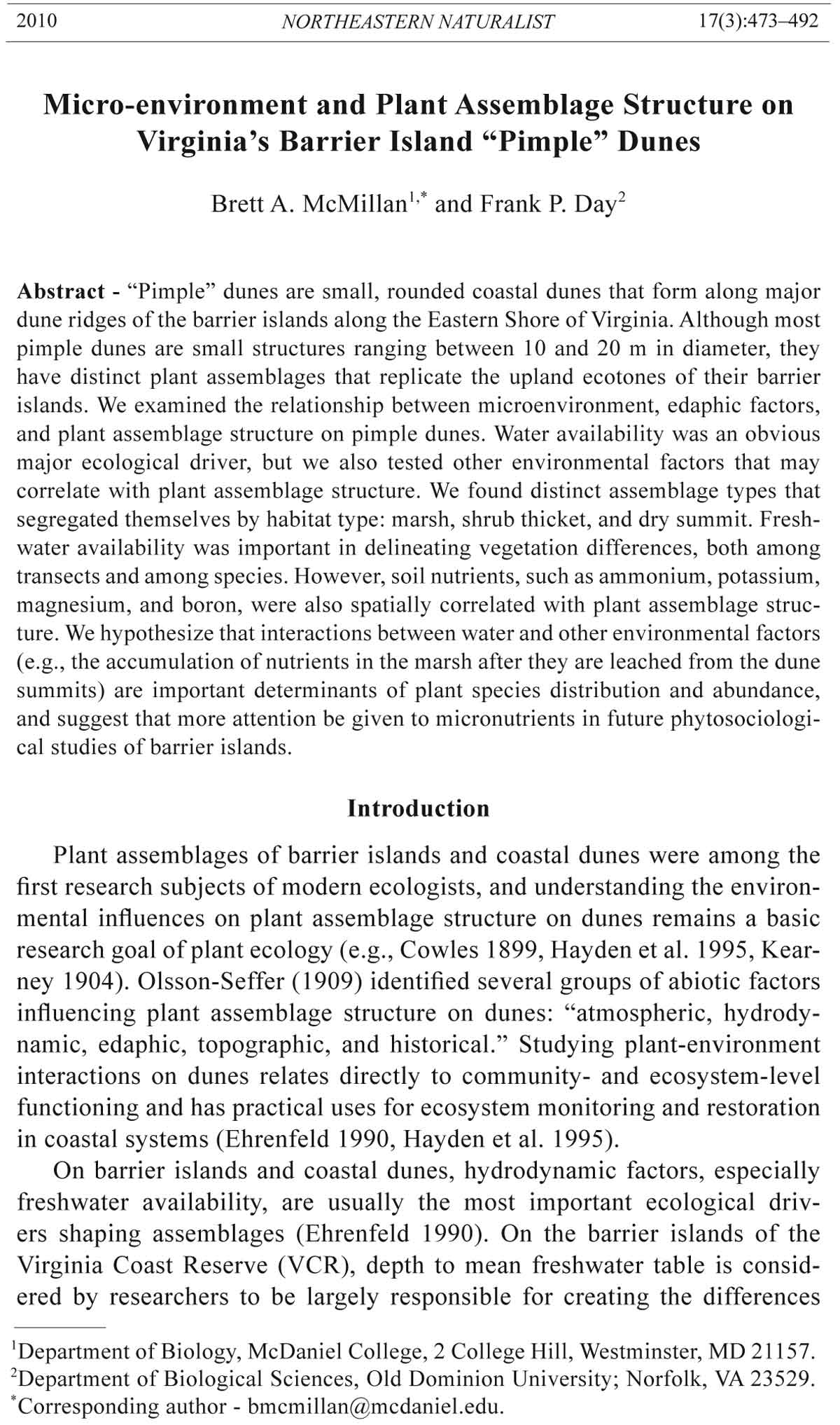
Rich 1934). The main dunes of the barrier island are typically laid down in
longitudinal rows by significant weather events, whereas pimples are circular
to slightly ovate and flat-topped (Fig. 1; Anthonsen et al. 1996, Cross
1964). There have been no conclusive studies about their formation, despite
a few hypotheses being posited (e.g., Cross 1964). We assume that they arise
from sand being deposited around pioneer plants, but the mechanism for how
that sand can be deposited in concentric circles is not clear. Pimple dunes
are typically 0.5–2 m taller than the elevation of the surrounding marsh, and
their diameters range from 5–25 m (Fig. 1).
Figure 1. Structural diagram of a pimple dune: A. Overhead view; B. Cross-section.
2010 B.A. McMillan and F.P. Day 475
The ecology of pimple dunes is not as well characterized as their geology,
but there have been some preliminary studies of their plant assemblages.
During the early years of research at the VCR Long-Term Ecological Research
(LTER) site, Hayden et al. (1995) noted that pimple dunes had clearly
delineated concentric zones that were readily distinguished by plant assemblages,
i.e., marsh graminoids, Morella cerifera (L.) Small (Wax Myrtle)
thickets, Iva frutescens L. (Marsh Elder) thickets, conifers, xeric forbs, and
graminoids. Similar assemblages occur along the inland elevation/water gradients
of the islands in much wider (100s of meters instead of 1–3 m) bands
that follow the lines of the main dunes.
We studied the relationships between plant assemblage composition
and microhabitat conditions to understand the environmental drivers that
create these tightly packed habitat zones. There have been many studies
of the synergistic effects between water table, soil, landscape, and biota
on plant assemblage composition, but there is no unified theory of plant
species-environment interactions as yet (Bazzaz 1996, Curtis and McIntosh
1951, Frego and Carleton 1995, Gauch 1982, Olsson-Seffer 1909,
Palmer 2010, Peet and Loucks 1977, Peet et al. 1988, Pielou 1984). Our
goals were to verify that water was indeed the most important ecological
driver shaping assemblages on the dunes and to describe what other
factors might be at play. We studied pimple dunes because they represent
simplified models of the inland ecosystem of the island, with sharply divided
plant assemblages.
We had three hypotheses: First, we expected that water availability
would be the most important factor determining assemblage structure on
pimple dunes. Second, we expected that soil variables other than water might
influence the distribution of plant species. Third, we expected that species
distributions may also be related to geomorphological features of the dune
system. In all three cases, we hoped to get both a broad view of species’
distributions as well as a finer view of how species with similar habitat preferences
partitioned themselves among microhabitats.
Field-site Description
We conducted this study on the pimple dunes of Hog Island, Northhampton
County, VA. Approximately 30 to 40 dunes on Hog Island lie
along a north–south line in the oldest interior swale marsh between two
dune ridges that formed in 1871 and 1955, respectively, with most pimple
dunes positioned closer to the 1955 ridge. We chose 17 pimples for our
study based on access to this line. The northwest and southeast corners of
the study were 37.454°N, 75.670°W and 37.446°N, 75.667°W (WGS84 datum),
respectively. We surveyed and marked permanent transects for annual
floristic surveys across the dunes during summer of 2003.
476 Northeastern Naturalist Vol. 17, No. 3
Methods
Floristic surveys
We designed our floristic sampling methods to begin to understand the
influence of the unique geomorphology of the dune system on vegetation
patterns. To maintain a constant elevation across the pimple dunes, we surveyed
plants using line transects instead of two-dimensional survey plots.
On each dune, there were three 5-m transects stratified among the three
assemblage zones: summit, shrubs, and marsh. Therefore, 51 transects (3
transects x 17 dunes) were laid out in total.
We defined assemblage types based on the growth habit of plant species
growing in them and on the amount of time that the types were routinely
inundated with water. Dry, sandy interiors with graminoids and forbs, but
few woody plants were defined as the summit. Sloping, dry to moist zones
with woody shrubs (mostly M. cerifera) were defined as shrub. The areas
within ≈2 m of the outer edge of the shrub canopy that were dominated by
marsh graminoids were defined as marsh.
The boundaries between assemblages were readily apparent and easily
distinguishable from both the growth habit of the plant species (e.g., graminoids
vs. woody plants) and their topographic setting (e.g., swale vs. dune
slope). Besides these large-scale differences, however, it was difficult to see
clearly defined patterns of individual species distributions, either in relation
to each other or to microhabitat. Morella cerifera was the only species found
on every dune, but most species were found in more than one assemblage
type. It was not apparent how habitat conditions other than elevation and
water availability varied between transects, if at all. Moreover, there was
overlap in the elevations, slopes, etc. between shrub and summit transects
on different pimples.
We conducted floristic surveys in June and July of 2003, 2004, and 2006
(logistical issues prevented a complete survey in 2005). We flagged the endpoints
of each transect and recorded coordinates for them so that the same
area could be measured each year. We made a collection of all plant species
encountered, and identified species using three floras for the region (Gleason
and Cronquist 1991, Radford et al. 1968, Weakley 2008). Each plant
species encountered was given an a priori habit-preference designation to
label them in ordination results: xerophytic, mesophytic, or hydrophytic. We
based these designations on the floras and field observations of the habitat
type where each species was usually encountered, but we had no preconceptions
about the edaphic or other microhabitat preferences of individual plant
species. Vouchers of all species recorded are deposited at the Old Dominion
University Herbarium.
Water availability
We measured the depth to the water table along each survey transect using
a soil auger to bore monitoring holes. The holes more or less remained
2010 B.A. McMillan and F.P. Day 477
open for the duration of the study, and could be re-checked with minimal
re-augering. Water levels were checked at each monitoring hole twice every
summer of 2003, 2004, and 2006 to determine the average range.
Soil variables
We measured a variety of soil properties. During the summers of 2005 and
2006, three soil cores collected at the middle and ends of each line transect
were mixed together (≈100 g total) to produce a composite soil sample. Subsamples
of the composite samples were extracted with 2N KCl solution, and
extracts were tested for ammonium and nitrate/nitrite concentration with a
Lachat colorimetric autoanalyzer at the Environmental Science Department
of the University of Virginia. Another set of subsamples was sent for analysis
at the Virginia Tech soil-testing laboratory. Each soil sample was tested for
pH, cation-exchange capacity (CEC), and nutrient concentrations (P, K, Ca,
Mg, Zn, Mn, Cu, Fe, and B). Organic matter was determined by mass loss
on ignition. Full descriptions of the chemical analyses are provided in Mullins
and Heckendorn (2005). Stratified samples collected during the initial
excavation of the water-table bore hole revealed that pimple dunes are made
of a well-sorted sand with little horizon development, and we therefore did
not use particle size as a factor. The thickness of the organic soil horizon was
measured at the bore holes.
Geomorphological features
We recorded physiographic variables for each transect. The elevation
of each transect above the mineral substrate was determined using a
surveying transit. We used the change in elevation and a plumb-bob inclinometer
to measure the percent slope of the ground within 1 m on either
side of the transect. We organized each of the three transects on each dune
along a radius line from the center of the dune to its periphery. This radius
had a random azimuth, so that we could investigate the influence of
aspect on plant assemblage and environmental conditions. Since aspect/
azimuth is recorded in degrees, a circular measurement, we converted it
to two linear variables, eastness and northness, using the sine and cosine
of the azimuth, respectively.
Statistical analyses
For the purpose of summarizing most environmental variables, we calculated
the mean ± 1 S.D. per assemblage type and tested for differences
between assemblages using parametric tests, i.e., ANOVA and ANCOVA.
Based on our first two hypotheses, it was important to account for the effect
of water-table depth on edaphic characteristics. We therefore tested
for assemblage effects (marsh vs. shrub vs. summit) on mean levels of
soil nutrients and other edaphic variables using mean water-table position
as a covariate in a one-way ANCOVA. We did not include dune identity as
a factor or block in the model since doing so reduced the residual degrees
of freedom too low for water-table position to be included as a covariate.
478 Northeastern Naturalist Vol. 17, No. 3
In a separate set of ANOVAs, however, in which pimple-dune identity was
included with assemblage in a full-factorial model, only three variables
exhibited a significant assemblage effect: potassium, potassium saturation,
and ammonium concentrations (see Results). We used repeated-measures
ANOVA to test for an assemblage effect on water table level and ANOVA to
test for differences in geomorphological variables; as with the edaphic variable
tests, we did not include a dune effect in the model.
To summarize the distribution of plant species among the assemblage
types, we calculated the annual mean species abundance along each transect.
If possible, we used ANOVA to determine if species distributions were influenced by the assemblage type. However, many species were not common
enough to use ANOVA to test whether assemblage type was significantly
related to their distribution. For the same reason, we could not examine the
influence of water-table level on most species distributions using ANCOVA
or linear regression. We therefore chose an alternate statistical method for
analyzing species distributions and environmental variables.
We primarily designed this study for analysis by ordination methods, because
typical parametric tests are not robust for data sets with many zeroes,
nor do they have the ability to evaluate relationships between all species
and environmental gradients simultaneously (McCune and Mefford 1999,
Pausas and Austin 2001, ter Braak 1986). Moreover, the primary goal of
ordination methods is to collapse a multivariate data set into fewer variables
so that patterns are more easily discernable (Palmer 2010).
Canonical correspondence analysis (CCA) is an ordination method
expressly designed to relate assemblage composition (i.e., combinations
of species abundances) to environmental factors (Kent and Ballard 1988,
Kourtev et al. 1998). The test creates regression relationships between all
variables in the species and environmental matrices. Those regression relationships
in turn are used in different combinations to produce mutually
orthogonal axes that explain a portion of the total variation between transects
or species (Gauch 1982, Kent and Ballard 1988). By convention, the axes are
ordered by the percentage of variation in the data that they explain; typically,
the amount of variation explained by each successive axis decreases rapidly,
so only the first two or three axes are usually examined for patterns (McCune
and Mefford 1999, Palmer 2010).
Plotting species or transects along a CCA axis creates a spatial representation
of statistical similarity or relatedness. For example, in an ordination
of transects, each transect is assigned a coordinate on the first axis, based
on both relative proportions of species and environmental variables. The numeric
distances between specific plant asemblages are measures of similarity
or relatedness between them. Assemblages farthest apart on the axis are the
most different. For that same axis, each environmental factor and species
also has a coordinate that can be thought of as a vector and represents the
relative contribution of that factor or species to the explanatory value of the
axis. Often, there will be groups of sample units (transects, in this example),
2010 B.A. McMillan and F.P. Day 479
whose connection may be surmised from the factors or species important to
the axis. Although the second axis was created using the same environmental
and species data as the first axis, it represents different combinations of
those data and is not correlated with the first. To tease out differences among
groups on the first axis, they may be plotted in a two-dimensional space using
the second axis.
We used two post-hoc tests from the CCAs to test our hypotheses. Monte-
Carlo resampling tests determine whether axes significantly described linear,
non-random relationships within the data matrices—i.e., whether CCAderived
patterns and associations are significantly different from random
ones (McCune and Mefford 1999). We also used Pearson’s correlation coefficients (r), which determine the percent contribution each variable made
towards the solution of each axis.
We ran CCA analyses in two different matrix configurations: 1) with
mean values of species abundances in each transect and mean values of environmental
characteristics in each transect and 2) with matrices transposed so
that we tested the average species cover per transect against the mean value
of environmental variables per species. To create this species-environmental
factors matrix, we calculated mean values of each environmental variable
from all transects in which a particular species occurred. The conventional
way to use CCA in studies like this one is with the first configuration (Palmer
2010), but we wanted to see if rearranging the matrices to focus on species
would reveal different patterns. Examining the analyses of the transect
matrix is still pertinent, however, because our field observations could not
discern differences in seemingly similar transects that were home to different
assemblage types. For example, there was variation within the range of
ca. 75 cm where the transition from shrub to summit assemblages started,
around the same as the range in pimple dune heights: 30–150 cm.
Results
Ordination overview
The transect matrix CCA and species matrix CCA explained 31% and
32%, respectively, of variation in the data with the first three axes of their
solutions (Table 1 and Figs. 2, 3). Each of the first three axes in both ordinations
explained 9–12% of variation in the data. In both ordination solutions,
relationships between variables and patterns were not random (Monte-Carlo,
P < 0.05 for all).
Assemblages: Water availability
Assemblage types had significantly different water levels (repeated-measures
ANOVA: F2, 29 = 72, P < 0.001; Table 2). Water-table position and its
direct correlate, elevation, were the two most important factors explaining
variation in plant species composition among transects (Pearson's r = 0.9
for the first axis in the transect CCA; Table 1). In the ordination, the tight
groupings formed by marsh transects indicated that they varied least among
480 Northeastern Naturalist Vol. 17, No. 3
Figure 2. Canonical correspondence analysis ordination of transects based on environmental
factors. Symbols represent transects; shapes indicate assemblage type. In
this and following figures, percentages listed on axes refer to the percentage of variation
explained. The percentages are cumulative and can be added to determine the
total percent of variation explained by both axes. The proximity of transect symbols
to each other on the two axes represents their similarity to each other based on the
environmental factors and species that occurred there. For example, the relatively
tight clustering of circles in the lower left indicates that marsh assemblages were
more similar in species composition and/or conditions than shrub and summit assemblages,
whose coordinates are more variable. Furthermore, the spacing of most
assemblages from marsh to shrub to summit along the first axis reflects the high
importance of water and elevation to Axis 1 (Table 1) and therefore represents a
moisture gradient between assemblages.
Table 1. Pearson’s correlation coefficients (r) for the five most important variables in the first
three axes of each CCA solution.
Transects
Axis 1: 12% Axis 2: 10% Axis 3:9 %
Variable r Variable r Variable r
Elevation 0.906 Mg -0.434 P -0.795
Water table -0.901 CEC -0.406 MgSat 0.694
O horizon -0.784 Ca -0.306 OM 0.646
CEC -0.540 Salinity -0.304 Fe 0.621
B -0.534 OM -0.295 Zn -0.597
Species
Axis 1: 12% Axis 2: 11% Axis 3: 9%
Variable r Variable r Variable r
K 0.567 NH4 0.536 Fe -0.380
KSat 0.552 O horizon 0.522 OM -0.345
MgSat -0.536 Water table 0.451 Mn -0.305
O horizon 0.486 Elevation -0.447 Slope 0.268
CEC 0.432 Mn -0.379 NOx 0.237
2010 B.A. McMillan and F.P. Day 481
the three assemblage types in terms of water availability, environmental
variables, and species composition (CCA; Fig. 2).
Assemblages: Soil variables
Although water availability was the most important factor associated
with the differences among plant assemblage types, some soil properties
were important as well. Concentrations of six soil elements: B, Cu, Fe, Mn,
P, and Zn, differed significantly among assemblage types (ANCOVA, for all
tests: F2,46 ≥ 7.8, P ≤ 0.001; Table 2); B, Ca, and Mg were associated with
water table depth (ANCOVA, for all tests: F1,46 ≥ 5.0; P ≤ 0.03; Table 2). B, P,
and Zn occurred in highest concentration in marsh transects, whereas Cu was
lowest in marsh habitat (Tukey’s: P < 0.01 for all). There was little NH4
+ or
NO3
- and no discernable pattern in nitrogen distribution among assemblage
types, but NH4
+, along with K and K base saturation, did exhibit a significant
difference in distribution among pimple dunes (Table 2). In terms of these
three variables, most dunes formed a single homogenous group, with two to
five dunes having significantly higher mean concentrations for NH4
+, K, and
K base saturation (Tukey's: P < 0.05 for all comparisons).
Table 2. Mean environmental conditions in pimple dunes by assemblage type ( ± 1 SD). CEC
= cation exchange capacity; meq = milliequivalents; OM = organic matter measured as loss
on combustion; Water = water table position relative to the marsh soil mineral horizon. For all
variables except water, the effect of assemblage type was tested with ANCOVA, using average
water-table position as covariate. Water-table position was tested with repeated measures
ANOVA. Italics = water-table position effect, F1,46 ≥ 5.0, P < 0.03; bold = significant assemblage
effect, F2,46 ≥ 12.5, P < 0.001; letters indicate significantly different groupings determined by
Tukey’s post-hoc test, P < 0.05. For assemblage effect with water table, F2,29 = 72, P < 0.001.
Asterisks indicate a significant pimple effect in an alternate ANOVA testing for pimple and assemblage
effects with interactions, F16,46 ≥ 5000, P < 0.01.
Marsh Shrub Summit Total
B (ppm) 0.6 ± 0.2a 0.3 ± 0.3b 0.14 ± 0.1c 0.34 ± 0.3
Ca (ppm) 224 ± 32 151 ± 110 91 ± 36 154 ± 87
Cu (ppm) 0.16 ± 0.05a 0.1 ± 0.01b 0.1 ± 0.02b 0.12 ± 0.04
Fe (ppm) 85 ± 20 134 ± 56 86 ± 35 102 ± 46
K (ppm)* 62 ± 103 88 ± 186 20 ± 11 57 ± 124
Mg (ppm) 111 ± 20 108 ± 64 51 ± 27 90 ± 50
Mn (ppm) 2 ± 0.5 2 ± 1 2 ± 1 2 ± 1
NH4 (ppm)* 94 ± 131 143 ± 255 90 ± 107 109 ± 175
NOx (ppm) 6 ± 12 10 ± 10 22 ± 23 13 ± 17
P (ppm) 25 ± 6a 11 ± 7b 14 ± 5b 16 ± 8
Zn (ppm) 1.7 ± 0.5a 1 ± 0.2b 1 ± 0.3b 1 ± 0.5
CEC (meq/100g) 2.2 ± 0.4a 1.9 ± 1.1b 0.9 ± 0.4c 1.6 ± 0.9
Casat (%) 52 ± 4 41 ± 11 50 ± 11 47 ± 10
Ksat (%)* 6 ± 7 7 ± 11 6 ± 3 6 ± 7
Mgsat (%) 42 ± 4 52 ± 9 44 ± 12 46 ± 9
OM (%) 0.9 ± 0.3 2.4 ± 1.3 1.1 ± 0.8 1.5 ± 1.1
Organic Horizon (cm) 9.8 ± 4.0a 7.9 ± 4.0a 3.0 ± 3.0b 6.8 ± 4.6
Water (cm) 11 ± 7a -17 ± 17b -51 ± 25c -19 ± 31
Elevation (cm) 22 ± 9a 54 ± 19b 84 ± 32c 54 ± 33a
482 Northeastern Naturalist Vol. 17, No. 3
2010 B.A. McMillan and F.P. Day 483
Species: Distribution among assemblages
The most abundant plant species exhibited measurable differences in
distribution among assemblage types, but most species did not restrict
themselves to assemblages that corresponded to their a priori habitat
preference designations (ANOVA: P < 0.05; Table 3). Morella cerifera
was the species with the highest amount of cover regardless of assemblage
type, with shrub zones having the most cover and summit transects the least
(Tukey’s: P < 0.0001; Table 3).
A large number of species were perennial graminoids. For example,
Distichlis spicata (L.) Greene (Saltgrass) was common in the marsh only
(Tukey’s: P < 0.0001; Table 3). Cover of Spartina patens (Aiton) Muhl.
(Saltmeadow Cordgrass), a C4 marsh grass, however was not significantly
different between marsh and summit plots (Tukey’s: P < 0.01; Table 3).
There were a few abundant perennial forbs as well, such as Polygonum hydropiperoides
Michx. (Waterpepper, Swamp Smartweed), which were more
abundant in the marsh and shrubs than in summit transects (Tukey’s: P <
0.01; Table 3).
Species: Water availability
Although water availability was the best predictor of differences between
assemblages, it was only one among many factors that were associated
with variation in the distribution and abundances of individual plant species
(Pearson's r = 0.4 for the second axis in the species CCA; Table 1).
Moreover, there was not as much variation in average water availability per
species as per transect assemblage type (Figure 3, cf. Table 2). Half of the
factors that were more important in the ordination (i.e., magnesium base
saturation, organic horizon thickness, cation exchange capacity; Table 1)
Figure 3 (opposite page). Canonical correspondence analysis ordination of species
based on environmental factors with overlays of environmental variables: A. water
availability overlay; B. soil potassium overlay; C. organic horizon depth overlay. In this
figure and Figure 4, symbols represent species, their shapes represent a priori habitat
preference, and their size represents the mean value of the particular variable across the
transects in which it was encountered. In the case of water, the variable is height of the
water table above the maximum depth, i.e., the bigger the symbol, the wetter the plot.
Each plot presents the same similarity data; i.e., species are in the same place in each
plot. The only difference between A, B, and C is that relative amounts of a particular environmental
variable are presented on top of the ordination data, hence the term “overlays”.
Species abbreviations are the same in this and Figure 4. ANDVIR = Andropogon
virginicus; BACHAL = Baccharis halimifolia; CYPSTR = Cyperus strigosus; DISSPI
= Distichlis spicata; EUPCAP = Eupatorium capillifolium (Lam.) Small (Dogfennel);
HYDVER = Hydrocotyle verticellata Thunberg (Whorled Marsh Pennywort); HYPHYP
= Hypericum hypericoides; HYPRAD = Hypochaeris radicata; IVAFRU = Iva
frutescens; PARQUI = Parthenocissus quinquefolia; PERPAL = Persea palustris;
PRUSER = Prunus serotina; SCIPNG = Scirpus pungens; SPAPAT = Spartina patens;
TOXRAD = Toxicodendron radicans P. Mill (Poison Ivy).
484 Northeastern Naturalist Vol. 17, No. 3
Figure 4 (opposite page). CCA of species based on environmental factors: A. ammonium
overlay; B. cation exchange capacity overlay; C. boron overlay. CIRHOR =
Cirsium horridulum Michx. (Yellow Thistle); EUPHYS = Eupatorium hyssopifolium
L. (Hyssopleaf Thoroughwort); JUNDIC = Juncus dichotomus Ell. (Forked Rush);
PANAMA = Panicum amarum; PANDIC = Panicum dichotomum (L.) Gould (Cypress
Panicgrass); PANIC1 = Panicum sp.; PANLAN = Panicum lanuginosum Ell. (Tapered
Panicgrass); PANLEU = Panicum leucothrix Nash (Rough Panicgrass); PANVIR
= Panicum virgatum; RUMACE = Rumex acetosella L. (Common Sheepsorrel);
SCHSCO = Schizachyrium scoparium. (for other species abbreviations, see Fig. 3).
did have a significant correlation with water in the parametric tests of assemblages
(Table 2).
Species: Soil variables
Soil conditions were the best predictors of individual species’ distributions;
the most important factors were potassium and potassium base
saturation, magnesium base saturation, depth of organic horizon, cation
exchange capacity, and soil ammonium (CCA; Figs. 3, 4). The distributions
of Iva frustescens L. (Jesuit's Bark), Persea palustris (Raf.) Sarg. (Swamp
Bay), and Hypochaeris radicata L. (Hairy Cat's Ear) were all influenced
Table 3. Mean percent cover per year, per transect, based on habitat type ( ± 1 SD) for the 20
species with highest average percent cover. Numbers in parentheses by habitat type are total
number of species encountered across five years. Key to superscripts: habit—F = forb, G =
graminoid, L = liana (i.e., woody vine), S = shrub, T = tree, and V = herbaceous vine; I =
introduced, NI = both native and non-native sub-species/genotypes. All herbaceous species
are perennial, and all species are native except as designated. Lowercase letters indicate significantly different groups based on habitat (ANOVA: F2,426 ≥ 3.1, P < 0.05; Tukey’s: P < 0.01);
Asterisks indicates insufficient data for parametric tests.
Species Marsh (27) Shrub (22) Summit (37)
Morella ceriferaST 59 ± 43b 100 ± 20a 67 ± 45b
Spartina patensG 14 ± 23a 0.2 ± 1.2b 8 ± 22a
Polygonum hydropiperoidesF 17 ± 29a 11 ± 24a 4 ± 14b
Mikania scandensV 3 ± 12a 1 ± 8b 0.5 ± 1.7c
Parthenocissus quinquefoliaL 1 ± 7a 11 ± 24b 2 ± 10a
Schoenoplectus pungensG 14 ± 30a 0.02 ± 0.17b 0.2 ± 0.9b
Juncus dichotomusG 0.04 ± 0.27 0.09 ± 0.62 4 ± 12
Festuca rubraGNI - 4 ± 12a 5 ± 12b
Ammophila breviligulataG - - 1 ± 5
Schizachyrium scopariumG - - 4 ± 11b
Rubus argutusS 0.04 ± 0.23a 0.2 ± 0.7ab 10 ± 19b
Panicum amarumG - - 0.9 ± 5
Baccharis halimifoliaST 3 ± 10a 1 ± 6.5b 0.4 ± 2.7c
Rumex acetosellafi- - 5 ± 15
Galium spp.F* 1 ± 3 1 ± 3 -
Eupatorium capillifoliumF* - - 1 ± 7
Dichanthelium sphaerocarponG* - 1 ± 2 1 ± 3
Phyla lanceolataF 0.7 ± 3a 0.06 ± 0.42b -
Eupatorium hyssopifoliumF* - - 2 ± 8
Hydrocotyle verticellataF 1 ± 8a 2 ± 9a 0.03 ± 0.14b
2010 B.A. McMillan and F.P. Day 485
486 Northeastern Naturalist Vol. 17, No. 3
by soil potassium and potassium base saturation—the two most important
variables in the species ordination and two of three variables that were
significantly different among individual dunes (Pearson's r > 0.5 for both
variables relative to the first CCA axis, Tukey’s: P < 0.05; Tables 1 and 3,
Fig. 4). These species were only encountered on one or two dunes that coincidentally
were among the few dunes exhibiting higher soil potassium.
Most species did not form cohesive groups in the ordination based on
our a priori habitat preference designations. A group of hydric and mesic
species including Cyperus strigosus L. (Strawcolored Flatsedge), Distichlis
spicata, Parthenocissus quinquefolia (L.) Planch. (Virgnia Creeper),
and Prunus serotina Ehrh. (Black Cherry) shared particularly thick organic
horizons (CCA, Pearson's r = 0.5; Fig. 3c). Other mesic and hydric species
not in this group, e.g., Hypericum hypericoides (L.) Crantz (St. Andrew's
Cross), Typha latifolia L. (Cattail), Ptilimnium capillaceum (Michx.) Raf.
(Herbwilliam/Bishopweed), and Andropogon virginicus L. (Bluestem),
were associated with relatively thinner soil organic horizons. There was a
similar pattern between species associations and soil ammonium (Fig. 4a).
All of the grass species in the genus Panicum were grouped in the same
area of the species ordination (Fig. 4a), despite being both mesic and xeric.
They appeared to have similar affinities for environmental variables, notably
magnesium base saturation.
There was a relatively tight group of xerophytes in the species ordination.
This group tended to be found in soil with relatively high cation
exchange capacity, with the exceptions of Panicum amarum Elliot (Bitter
Panicgrass), P. virgatum L. (Switchgrass), and Schizachyrium scoparium
(Michx.) Nash (Little Bluestem) (Fig. 4b). There was a similar pattern
with B, which, although of relatively minor importance in the species
ordination, was one of the top factors discriminating transects in the
transect ordination (Fig. 4c).
Spartina patens, the grass found in both marsh and dune summits, had
scores close to zero on the first three axes of the CCA. Being near the origin
of the ordination means that S. patens was intermediate in most of its habitat
preferences relative to other species.
Species: Geomorphological features
Of the geomorphological features used to describe species distributions
in the ordination, only elevation had a major impact (Table 1). The influence
of elevation, as measured by CCA, was nearly equal and opposite that of
the water table (Table 2; Pearson’s r = -0.47 and -0.45, respectively, for the
second axis; hydric species tended to associate with water availability and
xeric species with elevation. We performed a linear regression analysis of
the effect of elevation on water table and found the relationship to be strong
(R2 = 0.8, P < 0.0001). We therefore considered elevation a strong analog to
water table.
2010 B.A. McMillan and F.P. Day 487
Discussion
We found that distance to the water table was the best predictor of
plant assemblage on pimple dunes. It was not, however, the best predictor
of species found within any given assemblage, but rather one of several
variables. The factors most strongly associated with plant species distribution
were soil nutrients. Physiographic features such as slope and
aspect were not important.
Influence of water
As we hypothesized, water availability was the most important factor
determining assemblage type, based on both the direct results of the ordinations
and water being a significant covariate in many of the ANCOVAs. This
finding agrees with the long-held hypothesis about the importance of the
relative positions of the freshwater table and soil surface as an ecological
driver on the barrier islands (Hayden et al. 1995). Although water availability
is directly important for meeting the transpiration requirements of plants
and soil biota, it may also influence a host of other environmental factors that
could influence assemblage structure.
Most of the other variables that were significantly different between assemblage
types in the ANCOVA tests were also significant covariates with
water availability (Tables 1 and 3). Most of the important variables describing
transect variation in the ordination were also among those that covaried
with water availability, but CCA is designed to be robust in dealing with
correlated variables (Palmer 2010). Furthermore, water was not the most
important variable in the species ordination, and it was difficult to see a pattern
of influence between water and species (Fig. 3a). We concluded that the
influences of other environmental factors were not simply proxies for water
availability, with the exception of elevation. Our results suggest that edaphic
variables, especially mineral nutrient concentrations in the soil, are potential
secondary determinants of assemblage type. The nature of biogeochemical
cycles on barrier islands and the interactions between the water table and soil
nutrients lend support to this conclusion.
Influence of soil variables
According to our ANCOVA results, many soil properties differed significantly among assemblage types and were the most important variables
(besides water) in the ordinations of transects and plant species. These findings
support our second hypothesis with two concessions. First, most of
these variables were significantly correlated with water table and may more
or less be proxies for the effect of water. Second, this study was designed
to describe patterns and cannot show causation directly. Nevertheless, there
have been several studies supporting the influence of various soil nutrients
on vegetation structure in dunes (e.g., Gorham 1958; Hester and Mendelsohn
1990; Jones 1972, 1975; Lammerts et al. 1999, 2001). Our evidence is
488 Northeastern Naturalist Vol. 17, No. 3
correlational; we can only point out that some nutrients, e.g., K, are linked
to species distributions, and cannot conclude that those nutrients determine
species distributions. Our findings combined with previous studies led us to
re-examine our second hypothesis that soil conditions also shape assemblage
structure and suggest a modification. We propose that, on a broad scale, the
interactions of soil nutrients and soil organic matter with the water table
are an important determinant of species distributions. In other words, it is
not simply water availability that is important, but also how water affects
the availability of soil nutrients. We base the assumption that it is nutrients
affecting plant distribution, not vice versa, on our own observations and
the results of the studies we present below, but we acknowledge that only
experimentation could determine which is actually the case.
The interaction of weather, water, and soil nutrients on barrier islands
affects the availability and bioavailability of those nutrients and should
therefore affect the distribution of plants. Elements such as phosphorus,
boron, magnesium, and potassium often enter the ecosystem by being
deposited from salt spray (Boyce 1954, Bricker 1993). The uneven distributions
of mineral nutrients could be artifacts of deposition events, such as
storms. Once in the ecosystem, many nutrients are easily leached from sandy
summits and can accumulate in the marsh or anywhere with abundant
organic matter (Bardgett et al. 2001, Boyce 1954, Bricker 1993, Brooks
and DeWall 1976, Westman 1983, Willis and Yemm 1961). This process
supports our second hypothesis that soil chemistry is likely to influence the
creation of assemblage zones on pimple dunes as well as the distribution of
individual species.
Differences in availability of magnesium and calcium have been implicated
in dominance shifts and growth responses in dune species, some
of which are congeneric or identical to those found on the pimple dunes
(Clayton 1972, Hester and Mendelssohn 1990, Khedr and Lovett-Doust
2000, Willis and Yemm 1961). For example, fertilization of dunes with
macronutrients (N, P, K) and micronutrients (Ca and Mg, if severely
limited) elicited a shift in dominance from a beach-colonizing grass
(Ammophila sp.) to a generalist grass with higher nutrient requirements
(Festuca rubra L. [Red Fescue]) (Clayton 1972, Gorham 1958). Magnesium
and calcium-related alkalinity is important to growth of endangered
basiphilous swale species in the Netherlands; one of those species, Samolus
valerandi L. (Seaside Brookweed), is also a member of the Hog Island
marsh flora, albeit uncommon (Bekker et al. 1999, Lammerts et al. 2001,
Willis 1963). Finally, mineral cations, especially calcium, often form
complexes with soil organic matter, which is typically highest in wet soils
with low decomposition rates, and may become more or less bioavailable
depending on the nature of the complexes (Khedr and Lovett-Doust
2000). This characteristic of the cations could help explain the importance
of organic layer thickness in the ordinations.
2010 B.A. McMillan and F.P. Day 489
Potassium is generally considered unlikely to be limited in a coastal
system, but it does leach freely and forms complexes with organic matter
(Gorham 1958, Jones 1975, Lammerts, et al. 1999). It could have a potential
role to play in the toxicity of reduced species of iron and manganese in
anoxic marshes (Jones 1972, Willis 1963). It has been shown to influence
growth in some dune species, especially when input is limited by lack of
salt spray, which is the case for dunes in the sheltered interior of the island
(Boyce 1954, Clayton 1972, Gorham 1958, Hester and Mendelssohn 1990,
Jones 1975, Willis and Yemm 1961, Willis 1963). High levels of potassium
were only associated with a few species in the ordination (Fig. 3b), which
suggests that it is indeed limiting and that some species may have a high
demand for it. Lastly, potassium was one of the few soil variables important
in the species ordination that did not co-vary with water, suggesting
that its putative effect on species’ distributions may be independent of interaction
with the water table.
Ammonium may be another soil nutrient that influences species distributions
independent of water. Like potassium, ammonium did not significantly
co-vary with water, and both variables varied significantly among pimples
(Table 2). Unlike potassium, the species that were associated with it were
not all uncommon (Table 3, Fig. 4a). Furthermore, the species associated
with higher ammonium concentrations occurred in all three habitat types
(Fig. 4a). This result suggests that ammonium has a patchy distribution that
in turn influences the distribution of a subset of species that may have a
higher nitrogen demand.
Hyperacumulation of micronutrients in the freshwater marsh, such as
boron, could explain the dominance of many salt-tolerant species there.
Boron is toxic to most plants in amounts only ten times that of optimal
fertilizing concentrations (Brooks and DeWall 1976). Rozema et al.
(1992) demonstrated that six graminoid and forb halophyte species (including
a species of Spartina) were generally more tolerant of high levels
of boron than glycophytes, probably as an adaptation to the relatively
high concentration of boron in seawater. Although swales between dunes
on Hog Island are essentially freshwater marshes, many of the dominant
hydrophytes are salt tolerant or even facultatively halophytic, e.g.,
S. patens and D. spicata, as are some uncommon species, e.g., Typha angustifolia
L. (Narrowleaf Cattail) (Boyce 1954, Kearney 1904, Radford et
al. 1968, Rozema et al. 1992).
Influence of geomorphological features
The geomorphological variables other than elevation, slope, and aspect
(divided here into eastern and northern exposure), are essentially proxies for
other factors such as wind exposure and insolation. They have been shown to
influence plant assemblages on dunes (Willis and Yemm 1961); however, the
lack of importance of these factors in the ordinations suggests that pimples
are too protected from exposure to prevailing winds or salt spray for them
to make a difference. Thus, our third hypothesis was not supported (Olsson-
Seffer 1909).
490 Northeastern Naturalist Vol. 17, No. 3
Summary
As hypothesized, freshwater availability was an important factor delineating
changes in plant assemblages. Only a few species on the island, most
notably S. patens, demonstrate an ability to grow well in both wet and dry areas.
Although freshwater is a driving force behind the ecology of the islands,
our findings suggest that there are some recurring patterns with nutrients
and their distribution that can potentially explain assemblage structure and
species distribution on the pimple dunes. Species that can survive both inundated
and saline conditions, i.e., halophytic hydrophytes or vice versa,
may be at a competitive advantage for life in the swale marsh, despite it being
a freshwater system. Many of the woody mesic species were associated
with high CEC or soil organic matter, suggesting that they needed relatively
“rich” soils. Summit assemblages generally comprised species that can withstand
low nutrient retention, although some xeric species were associated
with high CEC soils or other nutrients. Therefore, water table, organic matter,
and nutrient availability in general are associated with differences among
assemblages, whereas differences in individual nutrient concentrations are
associated with species composition within assemblages.
Acknowledgments
Financial support was provided by subcontract 5-26173 through the University
of Virginia’s National Science Foundation LTER grant (NSF 0080381). Many thanks
are due the staff at the VCR LTER, my undergraduate assistants, and colleagues
who volunteered their time on the Islands. Drs. T. Crist, R. Colwell, and N. Gotelli
provided support for their statistical programs. Dr. R.D. Bray helped with species
identifications, oversaw the reposition of the plant voucher collection, and offered
editorial advice, as did S. Derosier.
Literature Cited
Anthonsen, K.L., L.B. Clemmensen, and J.H. Jensen. 1996. Evolution of a dune from
crescentic to parabolic form in response to short-term climatic changes: Rabjerg
Mile, Skagen Odde, Denmark. Geomorphology 17(1–3):63–77.
Bardgett, R.D., J.M. Anderson, V. Behan–Pelletier, L. Brussaard, D.C. Coleman, C.
Ettema, A. Moldenke, J.P. Schimel, and D.H. Wall. 2001. The influence of soil
biodiversity on hydrological pathways and the transfer of materials between terrestrial
and aquatic ecosystems. Ecosystems 4(5):421–429.
Bazzaz, F.A. 1996. Plants in Changing Environments: Linking Physiological, Population,
and Community Ecology. Cambridge University Press, Cambridge, UK.
Bekker, R.M., E.J. Lammerts, A. Schutter, and A.P. Grootjans. 1999. Vegetation
development in dune slacks: The role of persistent seed banks. Journal of Vegetation
Science. 10(5):745–754.
Boyce, S.G. 1954. The salt spray community. Ecological Monographs. 24(1):29–67.
Bricker, S.B. 1993. The history of Cu, Pb, and Zn inputs to Narragansett Bay, Rhode
Island as recorded by salt-marsh sediments. Estuaries 16(3):589–607.
Brooks, D.J., and A.E. DeWall. 1976. Boron concentration in Chesapeake Bay sediments,
paleosalinity, and baymouth uplift. Chesapeake Science 17(3):221–224.
2010 B.A. McMillan and F.P. Day 491
Clayton, J.L. 1972. Salt spray and mineral cycling in two California coastal ecosystems.
Ecology 53(1):74–81.
Cowles, H.C. 1899. The ecological relations of the vegetation on the sand dunes of
Lake Michigan (concluded). Botanical Gazette 27(3):167–202.
Cross, C.L. 1964. The Parramore Island mounds of Virginia. Geographical Review
54:502–515.
Curtis, J.T., and R.P. McIntosh. 1951. An upland forest continuum in the prairieforest
border region of Wisconsin. Ecology 32(3):476–496.
Dietz, R.S. 1945. The small mounds of the Gulf coastal plain. Science
102(2658):596–597.
Ehrenfeld, J.G. 1990. Dynamics and processes of barrier island vegetation. Reviews
in Aquatic Sciences 2(3, 4):437–480.
Frego, K.A., and T.J. Carleton. 1995. Microsite tolerance of four bryophytes in a
mature black spruce stand: Reciprocal transplants. Bryologist 98(4):452–458.
Gauch, H.G., Jr. 1982. Multivariate Analysis in Community Ecology. Cambridge
University Press, Cambridge, UK. 312 pp.
Gleason, H.A., and A. Cronquist. 1991. Manual of the Vascular Plants of Northeastern
United States and Adjacent Canada. 2nd Edition. New York Botanical Garden
Press, New York, NY. 910 pp.
Gorham, E. 1958. Soluble salts in dune sands from Blakeney Point in Norfolk. The
Journal of Ecology 46(2):373–379.
Hayden, B.P., R.D. Dueser, J.T. Callahan, and H.H. Shugart. 1991. Long-term research
at the Virginia Coast Reserve: Modeling a highly dynamic environment.
BioScience 41:310–318.
Hayden, B.P., M.C.F.V. Santos, G. Shao, and R.C. Kochel. 1995. Geomorphological
controls on coastal vegetation at the Virginia Coast Reserve. Geomorphology
13(1–4):283–300.
Hester, M.W., and I.A. Mendelssohn. 1990. Effects of macronutrient and micronutrient
additions on photosynthesis, growth parameters, and leaf nutrient
concentrations of Uniola paniculata and Panicum amarum. Botanical Gazette
151(1):21–29.
Jones, R. 1972. Comparative studies of plant growth and distribution in relation
to waterlogging: V. The uptake of iron and manganese by dune and dune slack
plants. Journal of Ecology 60(1):131–139.
Jones, R. 1975. Comparative studies of plant growth and distribution in relation to
waterlogging: VIII. The uptake of phosphorus by dune and dune slack plants.
Journal of Ecology 63(1):109–116.
Kearney, T.H. 1904. Are plants of sea beaches and dunes true halophytes? Botanical
Gazette 37(6):424–436.
Kent, M., and J. Ballard. 1988. Trends and problems in the application of classification
and ordination methods in plant ecology. Vegetatio 78:109–124.
Khedr, A.-H., and J. Lovett–Doust. 2000. Determinants of floristic diversity and vegetation
composition on the islands of Lake Burollos, Egypt. Applied Vegetation
Science 3(2):147–156.
Kourtev, P.S., J.G. Ehrenfeld, and W.Z. Huang. 1998. Effects of exotic plant species
on soil properties in hardwood forests of New Jersey. Water, Air, and Soil Pollution
105(1–2):493–501.
492 Northeastern Naturalist Vol. 17, No. 3
Lammerts, E.J., D.M. Pegtel, A.P. Grootjans, and A. van der Veen. 1999. Nutrient
limitation and vegetation changes in a coastal dune slack. Journal of Vegetation
Science. 10(1):111–122.
Lammerts, E.J., C. Maas, and A.P. Grootjans. 2001. Groundwater variables and vegetation
in dune slacks. Ecological Engineering 17(1):33–47.
McCune, B., and M.J. Mefford. 1999. Multivariate Analysis of Ecological Data. PC–
ORD for Windows version 4.1. MjM Software, Gleneden Beach, OR.
Melton, F.A. 1935. Vegetation and soil mounds. Geographical Review 25:431–433.
Mullins, G.L., and S.E. Heckendorn. 2005. Laboratory procedures. Publication
452-881. Virginia Tech Soil Testing Laboratory, Virginia Cooperative Extension,
Blacksburgh, VA.
Olsson-Seffer, P. 1909. Relation of soil and vegetation on sandy sea shores. Botanical
Gazette 47(2):85–126.
Palmer, M. 2010. The ordination web page: Ordination methods for ecologists. Oklahoma
State University, Stillwater. Available online at http://ordination.okstate.
edu. Accessed February 2010.
Pausas, J.G., and M.P. Austin. 2001. Patterns of plant species richness in relation
to different environments: An appraisal. Journal of Vegetation Science
12(2):153–166.
Peet, R.K., and O.L. Loucks. 1977. A gradient of southern Wisconsin forests. Ecology
58(3):485–499.
Peet, R.K., R.G. Knox, J.S. Case, and R.B. Allen. 1988. Putting things in order:
The advantages of detrended correspondence analysis. American Naturalist
131(6):924–934.
Pielou, E.C. 1984. The Interpretation of Ecological Data. John Wiley and Sons, New
York, NY.
Radford, A.E., H.E. Ahles, and C.R. Bell. 1968. Manual of the Vascular Flora of the
Carolinas University of North Carolina Press, Chapel Hill, NC. 1183 pp.
Rich, J.L. 1934. Soil mottlings and mounds in northeastern Texas as seen from the
air. Geographical Review 24:576–583.
Rozema, J., J. de Bruin, and R.A. Broekman. 1992. Effect of boron on the growth
and mineral economy of some halophytes and non–halophytes. New Phytologist
121(2):249–256.
ter Braak, C.J.F. 1986. Canonical correspondence analysis: A new eigenvector technique
for multivariate direct gradient analysis. Ecology 67(5):1167–1179.
Weakley, A.S. 2008. Flora of the Carolinas, Virginia, and Georgia, and surrounding
areas: Working draft of 7 April 2008. University of North Carolina
Herbarium, Chapel Hill, NC. Available online at http://herbarium.unc.edu/.
Accessed April 2009.
Westman, W.E. 1983. Island biogeography: Studies on the xeric shrublands of the
Inner Channel Islands, California. Journal of Biogeography 10(2):97–118.
Willis, A.J. 1963. Braunton Burrows: The effects on the vegetation of the addition of
mineral nutrients to the dune soils. Journal of Ecology 51(2):353–374.
Willis, A.J., and E.W. Yemm. 1961. Braunton Burrows: Mineral nutrient status of the
dune soils. Journal of Ecology 49(2):377–390.