Northeastern Naturalist 616 L.L. Mastro, D.J. Morin, and E.M. Gese 22001199 NORTHEASTERN NATURALIST 2V6(o3l). :2661,6 N–6o2. 83 Home Range and Habitat Use of West Virginia Canis latrans (Coyote) Lauren L. Mastro1,*, Dana J. Morin2,3, and Eric M. Gese4 Abstract - Canis latrans (Coyote) has undergone a range expansion in the United States over the last century. As a highly opportunistic species, its home range and habitat use changes with ecological context. Coyotes were first reported in West Virginia in 1950 but were not commonly observed until the 1990s, and there is scant information on Coyotes in the region. We used telemetry data from 8 radiocollared Coyotes in West Virginia to estimate home-range size and third-order habitat selection. Home-range areas (95% utilization distributions; UDs) varied from 5.22 to 27.79 km2 (mean = 12.48 ± 2.61 km2), with highly concentrated use of smaller core areas (mean 50% UD = 1.85 ± 0.34 km2), indicated by low flatness ratios (50% isopleths/95% isopleths varied from 0.11 to 0.20). Third-order habitat selection revealed most use was proportional to availability, although there was evidence of avoidance of disturbed /developed and riparian land cover at the 95% UD scale, and selection for softwood stands at both spatial scales when available. Our results provide preliminary space-use information for West Virginia Coyotes and suggest that although Coyotes are habitat generalists, space use in the region is not uniform, but instead concentrated in disjointed areas that are used intensively. Introduction Home-range movements and habitat selection can provide valuable insight into the behavior of individuals in a population including required and potentially impacted resources (Powell 2012). Canis latrans Say (Coyote) is a medium-sized, opportunistic, omnivorous, social carnivore, which has expanded its range and now occurs across most of North America (Bekoff and Gese 2003, Gompper 2002). The dietary and social plasticity of Coyotes and their ability to adapt to a broad range of habitats and conditions across different regions has facilitated this expansion (Crimmins et al. 2012). As a result, there is difficulty in predicting population responses to management actions and potential impacts to agricultural and natural resources in recently colonized areas of the Coyote’s range. Evaluating animal home ranges, or the area an individual requires to meet daily and seasonal resource needs, is a common method for describing space use of individuals within a population (Burt 1943). Coyotes are territorial, and the availability of undefended space can be a limiting factor in population regulation (Knowlton 1US Department of Agriculture, Animal and Plant Health Inspection Service, Wildlife Services, 105B Ponderosa Drive, Christiansburg, VA 24073. 2Cooperative Wildlife Research Laboratory, Southern Illinois University, 1125 Lincoln Drive, Carbondale, IL 62901. 3Current address - Department of Wildlife, Fisheries and Aquaculture, Mississippi State University, Box 9680, Mississippi State, MS 39762. 4US Department of Agriculture, Animal and Plant Health Inspection Service, Wildlife Services, National Wildlife Research Center, Utah State University, Logan, UT 84322.*Corresponding author - Lauren.L.Mastro@aphis.usda.gov. Manuscript Editor: Michael J. Cramer Northeastern Naturalist Vol. 26, No. 3 L.L. Mastro, D.J. Morin, and E.M. Gese 2019 617 and Gese 1995). Home-range size is dependent on availability and distribution of resources (Mills and Knowlton 1991, Patterson and Messier 2001), and Coyotes tend to have larger home ranges in areas where resources are sparse and spatially dispersed (Wilson and Shivik 2011). However, home-range size is also limited by the metabolic requirements of defending a territory (McNab 1963), and ideal despotic distribution predicts greater disparity in available resources will result in more intense competition among individual Coyotes for high-value territories (Andren 1990, Morin and Kelly 2017). When individuals are unable to establish and defend a territory (i.e., behave as a resident), they may become transients, occupying expansive home-range areas, or biding areas, commonly in suboptimal habitats and in the interstitial spaces between territories (Hinton et al. 2015, Kamler and Gipson 2000). Coyotes are commonly described as habitat generalists because they can occur in most habitat types (Chamberlain et al. 2000, Litvaitis and Harrison 1989), but there may still be differences in how individuals use habitat within their home range (third-order habitat selection; Johnson 1980). Habitat selection by Coyotes is typically attributed to prey or food availability (Boisjoly et al. 2010, Mills and Knowlton 1991), and studies in the eastern US suggest Coyotes select for open habitat types which are assumed to provide improved foraging capabilities (Cherry et al. 2016, Crête et al. 2001, Hinton et al. 2015, Richer et al. 2002, Ward et al. 2018). However, habitat selection and utilization by Coyotes can be highly variable and likely context dependent (Gosselink et al. 2003, Harrison et al. 1991, Parker and Maxwell 1989, Patterson and Messier 2001). The distribution of areas and resources selected or avoided can elucidate how Coyotes use space within their territories relative to high-value resources, threats from intraspecific competition, and risk of mortality (Monsarrat et al. 2013, Patterson and Messier 2001). Coyotes were first reported in West Virginia in 1950 (Taylor et al. 1976, Wykle 1999), and occurrences there continued to be sporadic until the 1990s (Wykle 1999). The West Virginia Division of Natural Resources reported an increase in the number of Coyote pelts sold from 1989 to 2017, but no other demographic information on Coyote populations in the state is currently available (R. Rogers, West Virginia Division of Natural Resources, Romney, WV, 2017 per comm.). Information on eastern Coyote home ranges and habitat use in the central Appalachians is also limited (Crimmins et al. 2012, Mastro 2011, Morin and Kelly 2017). We used telemetry data from 8 radio-collared Coyotes monitored across 16 counties to obtain preliminary baseline information on Coyote home-range size and third-order habitat selection in West Virginia. Field-site Description We captured Coyotes on the Stonewall Jackson Wildlife Management Area in Lewis County, and on private properties in Lewis, Nicholas, Pendleton, and Randolph counties in West Virginia. Radio-collared animals were monitored in Calhoun, Barbor, Fayette, Greenbrier, Harrison, Lewis, Upshur, Mercer, Monroe, Northeastern Naturalist 618 L.L. Mastro, D.J. Morin, and E.M. Gese 2019 Vol. 26, No. 3 Nicholas, Pendleton, Pocahontas, Randolph, Raleigh, Summers, and Webster counties. These counties lie within the Ridge and Valley and Appalachian Plateau physiographic provinces (Fenneman 1938). The Ridge and Valley is a long parallel series of uniform ridges interspersed with wide valleys that run northeast–southwest (Fenneman 1938). The Appalachian Plateau is a large, sloping plateau which has been dissected and eroded into various systems of mountains and valleys (Fenneman 1938). Elevations in the aforementioned counties vary from 184 m to 1400 m (USGS 1999). This wide range in elevation causes prevailing weather patterns to deposit anywhere from 152 cm of precipitation to less than half this amount per year on the region (USFS 2011). These climatic differences lead to a wide variety of ecological communities; high elevations are dominated by Picea rubens Sarg. (Red Spruce) forest typical of northern boreal forests, while low elevations are dominated by stands of mixed northern hardwoods and dry-site Quercus (oak) and Pinus strobus L. (Eastern White Pine) (USFS 2011). Methods Capture and monitoring We captured Coyotes using padded foot-hold traps (Victor #3 Softcatch, Lititz, PA). We checked traps each morning but did not set them when overnight temperatures were forecast to fall below 0° C. Upon capture, Coyotes were physically restrained with muzzles and hobbles during processing. We recorded each animal’s sex, weight, body condition, and age, which we determined by tooth wear (Gier 1968). We fitted each of the first 5 Coyotes captured with a store-on-board global positioning system (GPS) collar (Lotek, Newmarket, ON, Canada). We programmed collars to acquire locations at 3- or 4-hour intervals for 23 weeks and then drop-off. We fitted all subsequent captured Coyotes with both a GPS collar and an independent lightweight secondary very high frequency (VHF) collar (Advanced Telemetry Systems, Isanti, MN). We released Coyotes at the capture site. Capture and handling methods were reviewed and approved by the US Department of Agriculture, National Wildlife Research Center’s Institutional Animal Care and Use Committee (QA-1649). We monitored collars for VHF mortality signals from the ground using a hand-held receiver (Communication Specialists, Inc., Orange, CA) and a 3-element Yagi (AF Atronics, Inc., Urbana, IL) or a whip antenna (Laird Technology, Akron, OH), and from the air using a hand-held receiver and a fixed-wing aircraft fitted with a pair of 3-element Yagi antennas. We monitored the radio-collared Coyotes until the GPS collar dropped-off, a mortality event occurred, or radio contact was lost. Home range and habitat selection Although the total number of Coyotes was small, there was a high frequency of relocations for individual Coyotes (every ~3 hours for 2–6 months for each individual), and we were able to estimate utilization distributions using biased-random bridges (Benhamou 2011). Biased-random bridges (BRB) are a movement-based kernel estimator that considers not only the location of recorded points, but also the Northeastern Naturalist Vol. 26, No. 3 L.L. Mastro, D.J. Morin, and E.M. Gese 2019 619 time at which they were recorded. A trajectory is estimated based on the chronological order and amount of time between points. Unlike Brownian-bridges (Horne et al. 2007), the BRB method also estimates a diffusion parameter to infer likely direction of movement between points of relocation, instead of assuming unknown movement in between relocations is random. We visually identified and removed dispersal and pre-dispersal exploratory movements to ensure estimates appropriately reflected home range and not a transition to a transient stage or multiple home ranges over time. We estimated BRB activity utilization distributions (UD) for Coyotes for the total length of time that they were radio-collared using the ‘adehabitatHR’ package (Calenge 2006) in R (R Core Development Team 2015). We estimated home-range size for total (95% UD isopleths) and core (50% isopleths) home range. Because we used a kernel density estimator, 50% of the UD can be equivalent to 50% of the total area (a flat kernel distribution), or the distribution can be very peak ed, or consist of mul - tiple peaks that would cover a smaller area (the more concentrated the use, the more peaked the kernel density distributions and the smaller the estimated 50% core areas relative to the total home-range area). To quantify this relationship, we calculated a UD “flatness” ratio (core-area isopleth/total-area isopleth; Monsarrat et al. 2013) to compare degree of concentrated space use within a home range where a value of 0.53 is approaching uniform space use, and smaller values represent more concentrated use. In other words, lower flatness ratio values indicate increasingly smaller patches of core home-range use over the total home-range area. Visual inspection of plotted isopleths revealed several individuals with very patchy UDs consisting of multiple disjointed polygons distributed across a larger region (diffuse multimodal kernel density distributions). To quantify this pattern, we estimated the 95% minimum convex polygon (95% MCP) to describe the total area encompassing all observations for an individual during the time they were monitored. We did not use this metric as an estimate of home range, but as a way to compare the total area covered by an individual in the process of moving between all parts of its home range. We used land-cover types from the National Land Cover Database GAP analysis (USGS 2017) as a proxy for habitat, collapsing them into 8 general categories (Appendix A) to estimate third-order habitat selection. To estimate habitat selection ratios (Manly et al. 2002) at the third-order of selection, we masked the land-cover types with the 95% and 50% UD vertices to quantify available habitat for each individual’s home range and estimated selection ratios (wi; defined as use/availability) using the widesIII function in the ‘adehabitatHS’ package in R (Calenge 2006). We compared selection ratios for the global tracked population, where a selection ratio lss than 1 suggests greater use of a land-cover type proportional to availability, and less than 1 suggests less use proportional to availability. Results We captured and radio-collared 11 adult Coyotes (5 males, 6 females) from October 2009 to October 2011. However, we were only able to recover and Northeastern Naturalist 620 L.L. Mastro, D.J. Morin, and E.M. Gese 2019 Vol. 26, No. 3 download data from GPS-collars deployed on 8 of these animals (4 males, 4 females). The GPS-collars collected data during different intervals from October 2009 to January of 2012 (Table 1). Collars provided a total of 29 months of data (2–6 months per animal; Table 1). Percent of successful GPS location attempts varied from 46.37% to 66.52% (mean = 57.54) for individual Coyotes. Four of the GPS-collars were collected after the pre-programmed drop-off unit deployed at 23 weeks, while the other 4 were returned before the 23 weeks elapsed, when the animals were shot, snared, or trapped; radio contact was lost for 3 collars which we were unable to recover. Home range and habitat selection There was high individual variability in 95% UD home-range size (Table 1). Mean 95% UD home range was 12.48 ± 2.61 km2. Mean 50% UD core home range was 1.85 ± 0.33 km2. 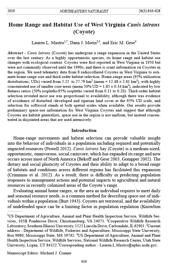The difference in 95% UD compared to the extent of the area covered by individuals (represented by MCPs) indicate that while Coyotes in the study area covered large swaths of land (95% MCP = 13.85–573.89 km2), use was relatively concentrated in smaller patches within the home range (Fig. 1). Low values of the estimated flatness ratios (0.11–0.20) further demonstrate the concentrated use of small areas within the 95% UD. Based on visual inspection, 6 Coyotes behaved as residents, appearing to maintain and defend stable territories over time, while 2 individuals displayed transient-like movements including shifting areas of use resulting in larger overall area encompassed (residents: 13.85 km2–28.73 km2, transients: 54.54 km2–573.89 km2). The proportions of available land cover were remarkably similar at both the 95% and 50% home-range level (Table 2). Mixed stands were the predominant land-cover type within Coyote home ranges (77.6%) and were used in proportion to availability at the 95% UD scale (wi = 1.04, 95% CI = 0.9–1.12). Selection ratios Table 1. Home-range metrics for Coyotes with GPS collars in West Virginia, October 2009–December 2011. Utilization distributions were estimated using biased-random bridges. Mean 95% utilization distribution (UD) was 12.48 km2 (± 2.61 SE) and mean 50% UD was 1.85 km2 (± 0.34). The UD “flatness” ratio (50% isopleth/95% isopleth; Monserrat et al. 2013) describes the degree of concentrated use. Flatness values approaching 0.53 represent uniform use of space, whereas lower values indicate more concentrated use of core areas. The 95% minimum convex polygons are not intended as a homerange estimate, but as a proxy for the total area covered by an individual during the time they were monitored. 95% 50% UD 95% UD UD flatness MCP Coyote (sex) Time range Relocations (km2) (km2) ratio (km2) c089 (M) October 2009–March 2010 858 16.50 1.88 0.11 28.73 c120 (M) December 2009–January 2010 255 5.22 0.85 0.16 54.54 c139 (F) December 2009–January 2010 274 10.38 2.00 0.19 24.93 c733 (M) May 2010–September 2010 605 7.65 1.46 0.19 13.85 c793 (F) May 2010–August 2010 410 16.02 3.22 0.20 22.21 c300 (M) June 2011–September 2011 585 8.74 1.27 0.15 14.61 c797 (F) June 2011–September 2011 488 27.79 3.28 0.12 573.89 c808 (F) November 2011–December 2011 227 7.58 0.85 0.11 17.82 Northeastern Naturalist Vol. 26, No. 3 L.L. Mastro, D.J. Morin, and E.M. Gese 2019 621 Figure 1. Plots of 50% (dark gray) and 95% (medium gray) utilization distributions for 8 Coyotes in West Virginia overlaid on 95% minimum convex polygons (MCP, light gray) showing concentrated home-range space use compared to patchy, diffuse home-range space use over much greater areas (c120 and c797). Note scale is not consistent between panels due to large differences in area. Northeastern Naturalist 622 L.L. Mastro, D.J. Morin, and E.M. Gese 2019 Vol. 26, No. 3 Table 2. Proportion of available land-cover types within 50% and 95% home-range utilization distributions (UD) and third-order habitat selection ratios (wi) for 8 Coyotes monitored in West Virginia from October 2009–December 2011, for duration of tracking. UD area/ Disturbed/ Mixed Metric Pasture developed Grass Hardwood stands Riparian Scrub Softwood 95% UD Proportion of available land-cover type 0.05 0.02 less than 0.01 0.04 0.84 0.04 less than 0.01 0.01 Third-order habitat selection ratios 1.05 0.41 1.58 1.01 1.04 0.52 1.59 1.40 (95% CI) (0.49–1.61) (0.25–0.57) (0.00–3.42) (0.94–1.08) (0.97–1.11) (0.33–0.71) (0.00–4.76) (1.18–1.63) 50% UD Proportion of available land-cover type 0.05 0.02 less than 0.01 0.04 0.86 0.03 less than 0.01 0.01 Third-order habitat selection ratios 1.04 0.47 1.89 0.80 1.01 0.74 1.25 2.16 (95% CI) (0.40–1.67) (0.00–1.46) (0.09–3.69) (0.27–1.32) (0.97–1.06) (0.33–1.14) (0.00–2.96) (2.16–2.16) Northeastern Naturalist Vol. 26, No. 3 L.L. Mastro, D.J. Morin, and E.M. Gese 2019 623 showed an avoidance of disturbed/developed (wi = 0.41, 95% CI = 0.25–0.57) and riparian (wi = 0.52, 95% CI = 0.33–0.71), and moderate selection of softwood stands (wi = 1.40, 95% CI = 1.18–1.63) at the 95% UD scale (Table 2). Selection ratios estimated at the 50% UD scale all overlapped 1 indicating use was proportional to availability, except for softwood stands, which were available and selected for by 1 individual at the core home-range scale (wi = 2.16). Discussion We found Coyotes in West Virginia had highly variable home-range sizes, although core-area sizes were relatively consistent. This is likely due to resource dispersion influencing the home-range area of each individual (Mills and Knowlton 1991, Wilson and Shivik 2001). The flatness ratios for all individuals indicated concentrated use of disproportionally small core areas, suggesting resources were clumped and territoriality may be a limiting factor (Morin and Kelly 2017, Windberg 1995, Windberg and Knowlton 1988). While data is preliminary, the space-use patterns observed are consistent with patterns reported previously in low-density Eastern Coyote populations in rural areas (Crête et al. 2001, Morin et al. 2016, Richer et al. 2002). Eastern Coyote home-range size can vary widely (Crête et al. 2001, Holzman et al. 1992, Person and Hirth 1991). Previous home-range estimates of eastern Coyotes have varied from 1.8 km2 (Crossett 1990) to 122.9 km2 (Crawford 1992) depending on region, habitat type, social structure, group size and hierarchical position, age, sex, season, and prey availability (Harrison and Gilbert 1985, Hinton et al. 2015, Parker and Maxwell 1989). The home ranges of Coyotes in the eastern United States are 100–200% larger than that of their western counterparts (Patterson and Messier 2001). However, generalizations about home range are difficult to make, not only due to the breadth of influencing factors, but also because methods of obtaining data and estimating home range differs between studies (Voigt and Berg 1987). Coyote home-range sizes are often negatively correlated with availability of resources (Hidalgo-Mihart et al. 2004, Mills and Knowlton 1991). Home-range size has repeatedly been found to decrease in areas of increasing human use and humanassociated habitat, with small home ranges in urban, suburban, or agriculturally fragmented landscapes, and larger home ranges in forested landscapes (Atwood et al. 2004, Crête et al. 2001, Gehrt 2007). Overall home-range sizes of Coyotes in our study were large compared to estimates from other regions, suggesting relatively low resource availability, but were consistent with the intermediate range of reported estimates for Coyotes in rural areas (Atwood et al. 2004). Despite relatively large home-range size and support for the effects of resource dispersion, there is some evidence to suggest competition for resources and territoriality influenced home-range use and movements in the region as it would in an established population. Six Coyotes behaved as residents, they regularly covered the entirety of their 95% MCP, and appeared to utilize the periphery of these areas more than the centers (Fig. 1). The consistently low Northeastern Naturalist 624 L.L. Mastro, D.J. Morin, and E.M. Gese 2019 Vol. 26, No. 3 flatness ratios demonstrated intensive use of core areas relative to total home range, suggesting much of the land cover within maintained home range (predominantly mixed forest) was suboptimal. Although there may be some bias in habitat selection ratios due to our fix acquisition rate (Frair et al. 2010), and additional research is needed, our findings were similar to other prior work. With the except of softwood stands, which appeared to be favored, Coyotes in our study selected for forested land-cover types proportional to availability, suggesting hardwood and mixed forests provide minimal resource value for Coyotes (Chamberlain et al. 2000, Crête et al. 2001, Crimmins et al. 2012, Morin 2015). Also similar to prior work, Coyotes avoided disturbed/developed areas at the 95% UD scale, indicating that Coyotes may be avoiding human activity at the third-order of selection (Atwood et al. 2004, Gehrt et al. 2009, Mitchell et al. 2015). Coyotes in our study avoided riparian land-cover types at the 95% UD scale similar to the findings of Hinton et al. (2015) but in contrast with those of other studies (Gosselink et al. 2003, Morin 2015, Sumner et al. 1984). We suspect that Coyotes may have avoided riparian areas in our study area because these areas represented increased association with humans (37.5% of Coyote home ranges were located in Stonewall Jackson Wildlife Management Area which includes a 1052-ha [2600-acre] lake and is adjacent to a State Park popular with outdoor recreationalists). While we can glean much from home range and habitat use of individual Coyotes, there are still many gaps in our knowledge of the West Virginia Coyote population. We can make assumptions about territory densities and spatially limiting factors, but we do not know overall population density, which can be largely influenced by prey, social structure, and rates of mortality (Messier and Barrette 1982, Morin et al. 2016). In addition, we do not know the local population response to mortality, including capacity for compensatory immigration, that would be critical for predicting the effect of management strategies (Kierepka et al. 2017, Morin and Kelly 2017). Overall, although our study suggests Coyote space use in West Virginia adheres to previously identified trends for Coyotes across their range, there are still many questions about local dynamics that would improve our ability to make informed management decisions. Acknowledgments This research was supported in part by the intramural research program of the US Department of Agriculture, Wildlife Services, National Wildlife Research Center; US Department of Agriculture, Wildlife Services-West Virginia and Virginia programs; and the West Virginia Division of Natural Resources. We thank the Civil Air Patrol – West Virginia Wing, individual landowners who allowed us access to their property, and individuals that returned collars. Michael Cramer and 2 anonymous reviewers provided constructive suggestions and comments on the manuscript. The findings and conclusions in this publication have not been formally disseminated by the US Department of Agriculture and should not be construed to represent any agency determination or policy. Northeastern Naturalist Vol. 26, No. 3 L.L. Mastro, D.J. Morin, and E.M. Gese 2019 625 Literature Cited Andren, H. 1990. Despotic distribution, unequal reproductive success, and population regulation in the jay Garrulus glandarius L. Ecology 71:1796–1803. Atwood, T.C., H.P. Weeks, and T.M. Gehring. 2004. Spatial ecology of Coyotes along a suburban-to-rural gradient. Journal of Wildlife Management 68:1000–1009. Bekoff, M., and E.M. Gese. 2003. Coyote (Canis latrans). Pp. 467–481, In G.A. Feldhamer, B.C. Thompson, and J.A. Chapman (Eds.). Wild Mammals of North America: Biology, Management, and Conservation, 2nd Edition. John Hopkins University Press, Baltimore, MD. 1216 pp. Benhamou, S. 2011. Dynamic approach to space and habitat use based on biased random bridges. PLoS ONE 6:e14592. Boisjoly, D., J.P. Ouellet, and R. Courtois. 2010. Coyote habitat selection and management implications for the Gaspésie caribou. Journal of Wildlife Management 74:3–11. Burt, W.H. 1943. Territoriality and home range concepts as applied to mammals. Journal of Mammalogy 24:346–352. Calenge, C. 2006. The package adehabitat for the R software: A tool for the analysis of space and habitat use by animals. Ecological Modelling 197:516– 519. Chamberlain, M.J., C.D. Lovell, and B.D. Leopold. 2000. Spatial-use patterns, movements, and interactions among adult Coyotes in central Mississippi. Canadian Journal of Zoology 78:2087–2095. Cherry, M.L., P.E. Howell, C.D. Seagraves, R.J. Warrant and L.M. Conner. 2016. Effects of land cover on Coyote abundance. Wildlife Research 43:662–670. Crawford, B.A. 1992. Coyotes in Great Smoky Mountains National Park: Evaluation of methods to monitor relative abundance, movement ecology, and habitat use. M.Sc.Thesis. University of Tennessee, Knoxville, TN. 72 pp. Crête, M., J.P. Ouellet, J.P. Tremblay, and R. Arsenault. 2001. Suitability of the forest landscape for Coyotes in northeastern North America and its implications for coexistence with other carnivores. Ecoscience 8:311–319. Crimmins, S.M., J.W. Edwards, and J.M. Houben. 2012. Canis latrans (Coyote) habitat use and feeding habits in central West Virginia. Northeastern Naturalist 19:411–420. Crossett III, R.L. 1990. Spatial arrangements and habitat use of sympatric Red Foxes (Vulpes vulpes) and Coyotes (Canis latrans) in central Kentucky. M.Sc.Thesis. Eastern Kentucky University, Richmond, KY. Fenneman, N.M. 1938. Physiography of Eastern United States. McGraw-Hill Book Company, New York, NY. 714 pp. Frair, J.L., J. Fieberg, M. Hebblewhite, F. Cagnacci, N.J. DeCesare, and L. Pedrotti. 2010. Resolving issues of imprecise and habitat-biased locations in ecological analyses using GPS telemetry data. Philosophical Transactions of the Royal Society 365:2187–2200. Gehrt, S.D. 2007. Ecology of Coyotes in urban landscapes. Proceedings of the 12th Wildlife Damage Management Conference 12:303–311. National Wildlife Research Center, Fort Collincs, CO. Gehrt, S.D., C. Anchor, and L.A. White. 2009. Home range and landscape use of Coyotes in a metropolitan landscape: Conflict or coexistence? Journal of Mammalogy 90:1045–1057. Gier, H.T. 1968. Coyotes in Kansas. Bulletin 393. Kansas State College of Agriculture and Applied Science, Agricultural Experiment Station, Manhattan, KS. 102 pp. Gompper, M.E. 2002. The ecology of northeast Coyotes: Current knowledge and priorities for future research. Wildlife Conservation Society, Bronx, NY. 47 pp. Northeastern Naturalist 626 L.L. Mastro, D.J. Morin, and E.M. Gese 2019 Vol. 26, No. 3 Gosselink, T.E., T.R. Van Deelen, R.E. Warner, and M.G. Joselyn. 2003. Temporal habitat partitioning and spatial use of Coyotes and Red Foxes in east-central Illinois. Journal of Wildlife Management 67:90–103. Harrison, D.J., and J.R. Gilbert. 1985. Denning ecology and movements of Coyotes in Maine during pup rearing. Journal of Mammalogy 66:712–719. Harrison, D.J., J.A. Harrison, and M. O’Donoghue. 1991. Predispersal movements of Coyote (Canis latrans) pups in eastern Maine. Journal of Mammalogy 72:756–763. Hidalgo-Mihart, M.G., L. Cantú-Salazar, C.A. López-González, E.C. Fernandez, and A. González-Romero. 2004. Effect of a landfill on the home range and group size of Coyotes (Canis latrans) in a tropical deciduous forest. Journal of Zoology 263:55–63. Hinton, J.W., F.T. van Manen, and M.J. Chamberlain. 2015. Space use and habitat selection by resident and transient Coyotes (Canis latrans). PLoS ONE 10:e0132203. Holzman, S., M.J. Conroy, and J. Pickering. 1992. Home range, movements, and habitat use of Coyotes in southcentral Georgia. Journal of Wildlife Management 56:139–146. Horne, J.S., E.O. Garton, S.M. Krone, and J.S. Lewis. 2007. Analyzing animal movements using Brownian bridges. Ecology 88:2354–2363. Johnson, D.H. 1980. The comparison of usage and availability measurements for evaluating resource preference. Ecology 61:65–71. Kamler, J.F., and P.S. Gipson. 2000. Space and habitat use by resident and transient Coyotes. Canadian Journal of Zoology 78:2106–2111. Kierepka, E.M., J.C. Kilgo, and O.E. Rhodes. 2017. Effect of compensatory immigration on the genetic structure of Coyotes. Journal of Wildlife Management 81:1394–1407. Knowlton, F.F., and E.M. Gese. 1995. Coyote population processes revisited. Pp. 1–6, In D. Rollins, C. Richardson, T. Blankenship, K. Canon, and S. Henke (Eds.). Symposium Proceedings - Coyotes in the Southwest: A Compendium of Our Knowledge. Texas Parks and Wildlife Department, Austin, TX. 180 pp. Litvaitis, J.A., and D.J. Harrison. 1989. Bobcat–Coyote niche relationships during a period of Coyote population increase. Canadian Journal of Zoology 67:1 180–1188. Manly, B.F., L.L. McDonald, D.L. Thomas, T.L. McDonald, and W.P. Erickson. 2002. Resource Selection by Animals: Statistical Design and Analysis for Field Studies. 2nd Edition. Kluwer Academic, Boston, MA. 221pp. Mastro, L.L. 2011. Life history and ecology of Coyotes in the Mid-Atlantic states: A summary of the scientific literature. Southeastern Naturalist 10:72 1–730. McNab, B.K. 1963. Bioenergetics and the determination of home-range size. The American Naturalist 97:133–140. Messier, F., and C. Barrette. 1982. The social system of the Coyote (Canis latrans) in a forested habitat. Canadian Journal of Zoology 60:1743–1753. Mills, L.S., and F.F. Knowlton. 1991. Coyote space use in relation to prey abundance. Canadian Journal of Zoology 69:1516–1521. Mitchell, N., W.F. Strohbach, R. Pratt, W.C. Finn and E.G. Strauss. 2015. Space use by resident and transient Coyotes in an urban–rural landscape mosaic. Wildlife Research 42:461–469. Monsarrat, S., S. Benhamou, F. Sarrazin, C. Bessa-Gomes, W. Bouten, and O. Duriez. 2013. How predictability of feeding patches affects home range and foraging habitat selection in avian social scavengers? PLoS ONE 8:e53077. Morin, D.J. 2015. Spatial ecology and demography of eastern Coyotes (Canis latrans) in western Virginia. Ph.D. Dissertation. Virginia Polytechnic Institute and State University, Blacksburg, VA. 186 pp. Northeastern Naturalist Vol. 26, No. 3 L.L. Mastro, D.J. Morin, and E.M. Gese 2019 627 Morin, D.J., and M.J. Kelly. 2017. The dynamic nature of territoriality, transience, and biding in an exploited Coyote population. Wildlife Biology wlb-00335. Morin, D.J., M.J. Kelly, and L.P. Waits. 2016. Monitoring Coyote population dynamics with fecal DNA and spatial capture–recapture. Journal of Wildlife Management 80:824–836. Parker, G.R., and J.W. Maxwell. 1989. Seasonal movements and winter ecology of the Coyote, Canis latrans, in northern New Brunswick. Canadian Field Naturalist 103:1–11. Patterson, B.R., and F. Messier. 2001. Social organization and space use of Coyotes in eastern Canada relative to prey distribution and abundance. Journal of Mammalogy 82:463–477. Person, D.K., and D.H. Hirth. 1991. Home range and habitat use of Coyotes in a farm region of Vermont. Journal of Wildlife Management 55:433–441. Powell, R.A. 2012. Diverse perspectives on mammal home ranges or a home range is more than location densities. Journal of Mammalogy 93:887–889. R Core Development Team. 2015. R: A language and environment for statistical computing. R Foundation for Statistical Computing, Vienna, Austria. Available online https:// www.R-project.org/. Accessed 12 February 2015. Richer, M.C., M. Crête, J.P. Ouellet, L.P. Rivest, and J. Huot. 2002. The low performance of forest versus rural Coyotes in northeastern North America: Inequality between presence and availability of prey. Ecoscience:44–54. Sumner, P.W., E.P. Hill, and J.B. Wooding. 1984. Activity and movements of coyotes in Mississippi and Alabama. Proceedings of Annual Conference of Southeast Association of Fish and Wildlife Agencies 38:174–181. Taylor, R.W., C.L. Counts III, and S.B. Mills. 1976. Occurrence and distribution of the Coyote, Canis latrans Say, in West Virginia. Proceedings of the West Virginia Academy of Sciences 48:3–4. US Forest Service (USFS). 2011. 2006 revised Monongahela National Forest land and resources management plan: Updated 2011. US Department of Agriculture, Washington, DC. 259 pp. US Geological Survey (USGS). 1999. National elevation dataset. Available online at http:// ned.usgs.gov/. Accessed 24 August 2012. USGS. 2017. National Gap Analysis Program (GAP) land cover data set. Available online at https://gapanalysis.usgs.gov/gaplandcover/data/. Accessed 15 January 2017. Voigt, D.R., and W.E. Berg. 1987. Coyote. Pp. 345–357, In M. Novak, J.A. Baker, M.E. Obbard, and B. Malloch (Eds.). Wild Furbearer Management and Conservation in North America. The Ontario Trappers Association and Ontario Ministry of Natural Resources, Totonto, ON, Canada. 1150 pp. Ward, J.N., J.W. Hinton, K.L. Johannesen, M.L. Karlin, K.V. Miller and M.J. Chamberlain. 2018. Home-range size, vegetation density, and season influences prey use by Coyotes (Canis latrans). PLoS ONE 13(10): e0203703. Wilson, R.R., and J.A. Shivik. 2011. Contender pressure versus resource dispersion as predictors of territory size of Coyotes (Canis latrans). Canadian Journal of Zoology 89:960–967. Windberg, L.A. 1995. Demography of a high-density Coyote population. Canadian Journal of Zoology 73:942–954. Windberg, L.A., and F.F. Knowlton. 1988. Management implications of Coyote spacing patterns in southern Texas. Journal of Wildlife Management 52:632–640. Wykle, J. 1999. The status of the Coyote, Canis latrans, in West Virginia. M.Sc. Thesis. Marshall University, Huntington, WV. 131 pp. Northeastern Naturalist 628 L.L. Mastro, D.J. Morin, and E.M. Gese 2019 Vol. 26, No. 3 Appendix A. Collapsed land-cover types and National Land Cover Database (NLCD) GAP habitat classifications. Collapsed land-cover types NLCD GAP classifications Pasture Cultivated Cropland Pasture/Hay Disturbed/developed Developed, High Intensity Developed, Low Intensity Developed, Medium Intensity Developed, Open Space Disturbed, Non-specific Grass Harvested Forest – Grass/Forb Regeneration Introduced Upland Vegetation – Annual Grassland Southern Appalachian Grass and Shrub Bald Hardwood stands Central and Southern Appalachian Montane Oak Forest North-Central Interior Wet Flatwoods Northeastern Interior Dry-Mesic Oak Forest Southern Appalachian Northern Hardwood Forest Mixed stands Allegheny-Cumberland Dry Oak Forest and Woodland - Hardwood Appalachian Hemlock-Hardwood Forest Central Appalachian Alkaline Glade and Woodland Central Appalachian Oak and Pine Forest Central Appalachian Pine-Oak Rocky Woodland Introduced Upland Vegetation - Treed Managed Tree Plantation Northeastern Interior Dry Oak Forest - Mixed Modifier Northeastern Interior Dry Oak Forest - Virginia/Pitch Pine Modifier Northeastern Interior Dry Oak Forest-Hardwood Modifier South-Central Interior Mesophytic Forest Southern and Central Appalachian Cove Forest Southern Ridge and Valley Dry Calcareous Forest Riparian Central Interior and Appalachian Floodplain Systems Central Interior and Appalachian Riparian Systems Central Interior and Appalachian Swamp Systems Open Water (Fresh) Ruderal Wetland Scrub Appalachian Shale Barrens Central Interior Calcareous Cliff and Talus Central Interior Highlands Calcareous Glade and Barrens Softwood stands Central and Southern Appalachian Spruce-Fir Forest Southern Appalachian Montane Pine Forest and Woodland